Particle basis function in the CPDI method

The Convected Particle Domain Interpolation (CPDI) method for evaluating nodal integrals in the weak form of the momentum equation employs a dynamically adaptive alternative to standard shape functions on the grid. The CPDI basis functions change depending on the underlying particle morphology. The animations in this post each provide image triplet groupings, one triplet for pure translation and the other for uniform stretching, defined as follows:

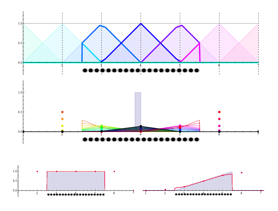
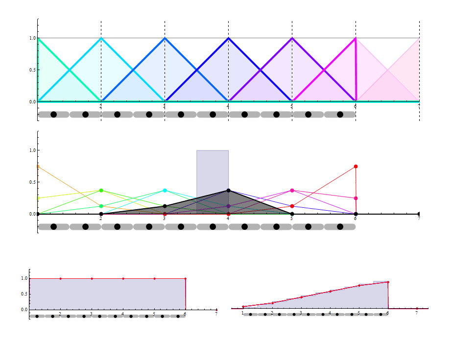
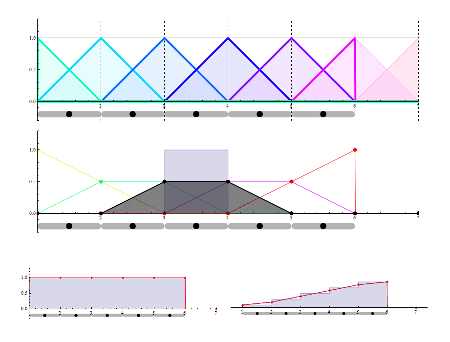
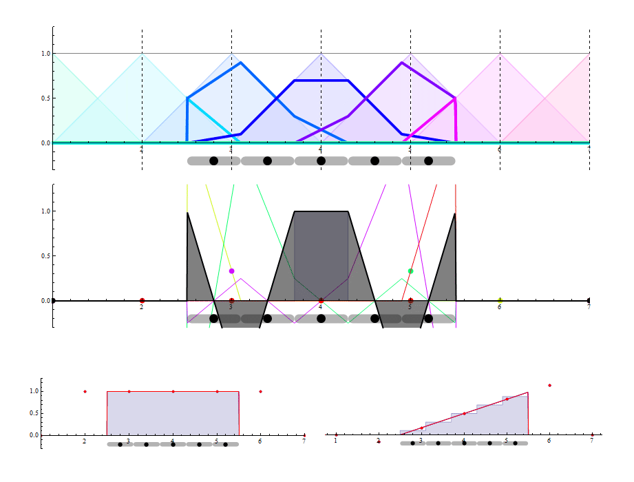
TOP IMAGE: The dynamic CPDI basis (solid lines) compared with the conventional FEM-style basis functions (shaded tent functions). The adaptive CPDI basis is constructed to exactly coincide with the conventional FEM basis at particle edges (called corners), and it varies linearly across each particle domain, thus making integrals of the basis or its gradient over a particle domain quite simple. The CPDI basis is linearly complete.
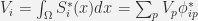
MIDDLE IMAGE: The particle basis (shown shaded in dark gray). Like the CPDI basis itself, the particle basis is never constructed explicitly. We are visualizing it here to better understand the domain of influence of a particle and (we hope) to discourage the mysterious tendency for researchers to refer to as the particle basis function. To the contrary, and as explained in detail in the bottom of this post, the particle basis function is the coefficient of the particle data value appearing in an expansion of a field as it is used in the discretization of governing equations. The solution of the governing equations uses a mapping of particle data to the grid. Consequently, because all fields are treated as expansions on the grid, the particle basis function (found by setting the particle value to 1 and all other particle data to zero) must be a grid expansion (so it MUST be piecewise linear on the grid if using linear shape functions). This proper definition of the particle basis function is shown below in dark gray. The particle basis function is NOT the top hat function (shown in light gray), nor is it as commonly and misleadingly asserted. The relatively complicated derivation of the particle basis function is provided at the bottom of this post. In the images below, two options are considered for the mapping particle data to the grid nodal value :
- Option 1: $\psi_{pi}^*=\frac{\phi_{ip}^*}{\sum_p\phi_{ip}}$
- Option 2: $\psi_{pi}^*$ is taken as the pseudo-inverse of $\phi_{ip}^*$

Here, $\phi_{ip}^*$ is the average of the ith CPDI grid nodal basis function, $S_i^*(x)$ over the pth particle domain $\Omega_p$ . The GIMP variants of MPM are similar except that they evaluate $\phi_{ip}$ and $\psi_{pi}$ using the conventional $S_i(x)$ grid basis functions rather than the adaptive (and actually computationally simpler) ones used in CPDI. Legacy “standard” MPM evaluates $\phi_{ip}$ to merely equal $S_i(x_p)$ , which causes grid-crossing errors. The figure groupings below use the CPDI formula $\phi_{ip}=\frac{1}{V_p}\int_{\Omega_p}S_i^*(x) dx$ in which $S_i^*(x)$ is the CPDI adaptive grid basis. The MIDDLE image in each image triplet shows the particle basis, which is constructed by applying the above mapping to the grid with all particle values set to 0 except 1 at the particle of interest. The light grey filled box in the middle image shows a piecewise constant description (=1 on the particle domain and 0 elsewhere), while the dark filled function is the associated particle basis on the grid. The dots show nodal values of the particle basis function to emphasize that nodal values are not equal to field values (there is no need for them to be). Seeing a nodal value “pop up” gives you a sense of when a particle begins to influence the field in grid cells containing that node. The other (colored) graphs in that plot are the similarly constructed basis functions for the other particles. As seen in the upcoming plots, OPTION 2 (the pseudo-inverse) produces particle basis functions that are neither positive everywhere nor of compact support (which could be problematic for parallelisation in applications).

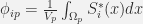
The BOTTOM row in each grouping of plots shows the representations of a field that is constant (at particles) and a field that linearly varying from 0 to 1 over the physical domain (with particle values set equal to that field at the particle location). As seen, OPTION 2 for setting $\psi_{pi}^*$ gives excellent results for the linear field when there are at least two particles per cell, but OPTION 1 seems to be a better overall choice because it gives good results for any particle density, including fractional particles per cell (desired for coarse descriptions in regions of little interest). Grid errors at boundaries with OPTION 1 could probably be reduced by enriching boundary particles (as described in the CPDI2 publication), but this remains to be proved.

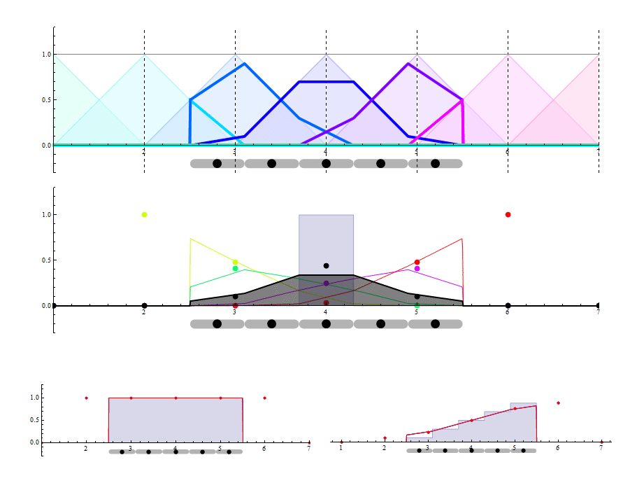
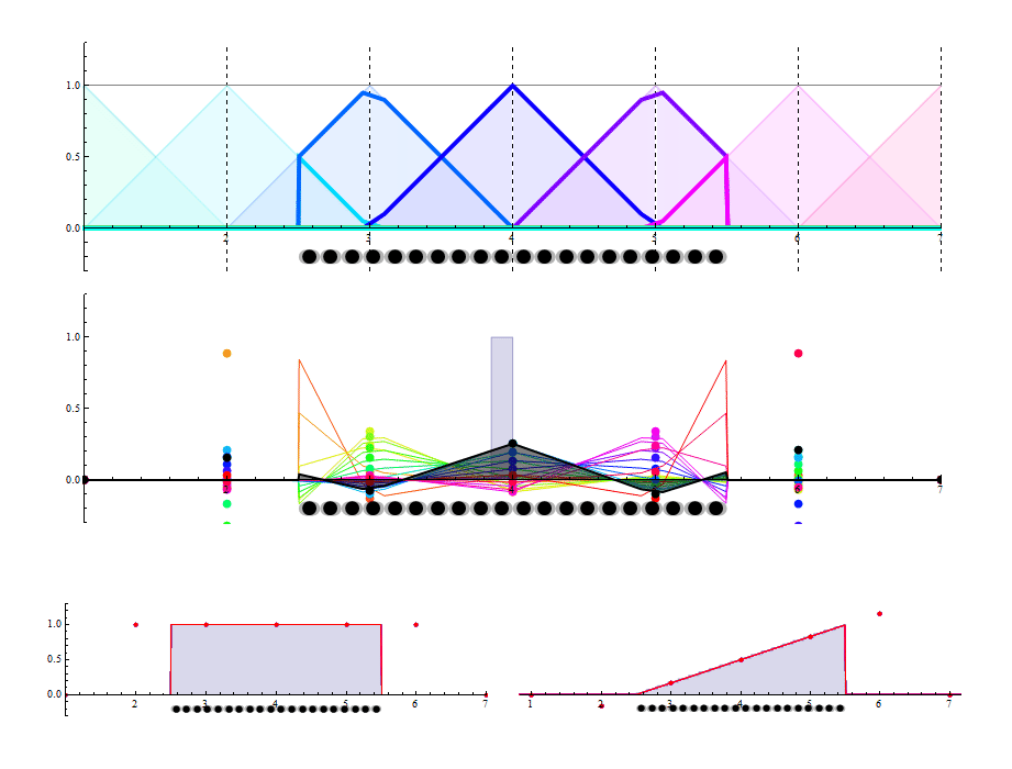
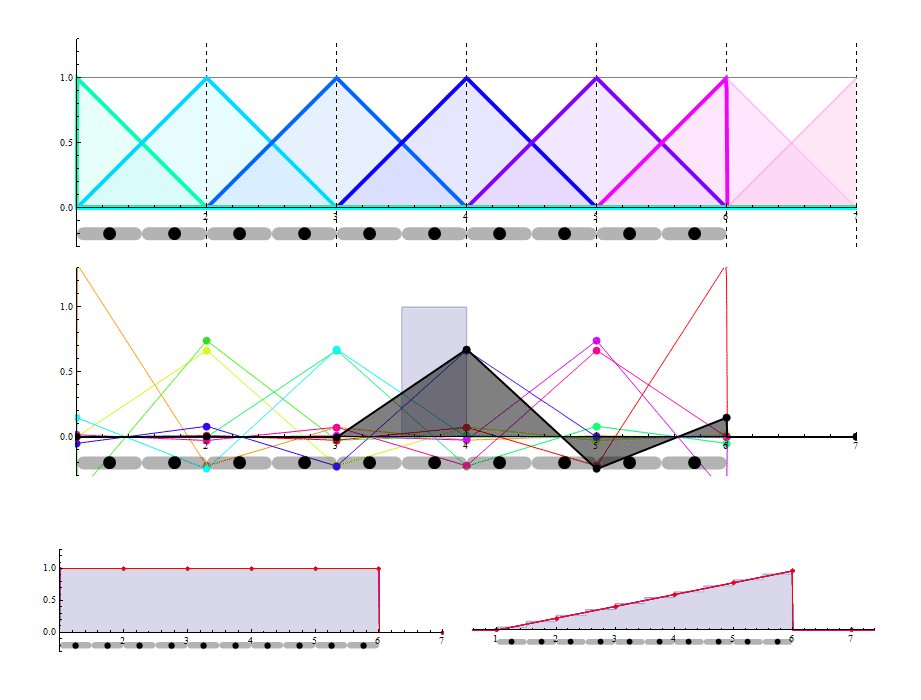
Results using OPTION 1

4 particles per cell (click on image if it seems to be low resolution or if it is not already animated). The light-gray box is a “tophat” function corresponding to all particle data being zero, except 1 at that selected particle. The dark gray function is the corresponding particle basis function that is used implicitly in the weak form of the momentum equations and which, therefore, is the right one to consider when proving that MPM is indeed a Partition of Unity (PoU) method. See bottom of post for the proof.
2 particles per cell
1 particle per cell
1/2 particle per cell (this one has the same particle size as above, but the grid density is doubled to give at least a few interior particles)

Results using OPTION 2

4 particles per cell
2 particles per cell
1 particle per cell
1/2 particle per cell

DERIVATION OF THE PARTICLE BASIS FUNCTION

Suppose that some function $u(x)$ is needed in the weak form of the momentum equation (or for any other purpose for which a full field is needed). This function is discretized on the grid as

$u(x)=\sum_i u_i^{*} S_i^{*}(x)$ ,

where $u_i^*$ is determined from particle data according to

$u_i^{*} =\sum_p \psi_{pi}^{*} u_p$

Combining these equations gives

$u(x)=\sum_p u_p^{*} b_p(x)$

where $b_p(x)$ is the particle basis function, defined by

$b_p(x)=\sum_i \psi_{pi}^{*} S_i^{*}(x)$

This satisfies partition of unity (PoU) only if, for all x in the body, $\sum_p b_p(x)=1$ . If the $\phi_{pi}$ are defined according to option 1 (which is what is used in all MPM formulations to our knowledge), then it follows that

$\sum_p \psi_{pi}^*=1$

Therefore, in this case,

$\sum_p b_p(x)=\sum_i S_i^{*}(x)=1$

In other words, the the particle basis functions satisfy partition of unity as long as the $S_i^{*}(x)$ grid basis functions satisfy partition of unity. For non-CPDI formulations, such as GIMP, there are errors in the evaluation of the $\psi_{pi}$ values arising from the fact that the integrals that must be theoretically taken over complicated particle domain shapes are actually taken over rectangles. In CPDI, this error is drastically reduced, but the particle domains still have gaps and overlaps that require discretization refinement to eliminate. In the limit as the discretization is refined, the gaps and overlaps disappear, thus ensuring that partition of unity is satisfied in the limit. This is why MPM formulations converge.

Comment: existence of gaps is not unique to MPM. Even FEM formulations have gaps and overlaps of the discrete tessellation in comparison to the actual body shape (where, for example, a curved boundary is treated as piecewise linear). The difference is that FEM has these only at the boundary, while MPM has them even in the interior. The effect is very small and diminishes with refinement for both FEM and MPM.

COMMENT.
Publications about MPM do not mention $\psi_{pi}$ , but it is lurking under the surface. MPM publications mention only $\phi_{ip}$ . However, the $\psi_{pi}$ is implicitly in the formulations to represent the mapping matrix for INTENSIVE specific (per unit mass) fields. For example, material velocity $v(x)$ may be interpreted as the INTENSIVE field “momentum per unit mass,” where momentum, $m v$ is the corresponding EXTENSIVE (non-field) lumped quantity. The momentum may be lumped at the nodes $(m_i v_i)$ or at the particles $(m_p v_p)$ . MPM formulations assign nodal momentum according to

$m_i v_i=\sum_p \phi_{ip} m_p v_p$
where $m_i=\sum_p\phi{ip}m_p$

In other words, solving for the nodal velocity,

$v_i=\sum_p \psi_{ip} v_p$
where $\psi_{ip}= \frac{\phi_{ip} m_p}{\sum_p\phi{ip}m_p}$

Thus, in these examples, for which all particles have the same mass $m_p$ , this formula for the INTENSIVE velocity field is equivalent to OPTION 1.

If it is desired to map a per-volume field $\sigma(x)$ to the grid, then it may be converted to a per-mass field by dividing by density. For example, grid values of stress (which has units of energy per volume) can be computed by using the mass-weighted average,

$\frac{\sigma_i}{m_i/V_i}=\sum_p \psi_{pi} \frac{\sigma_p}{m_p/V_p}$ ,
where $V_i=\int_{\Omega}S_i^*(x)dx=\sum_p V_p \phi_{ip}^*$

solving for $\sigma_i$ gives

$\sigma_i=\sum_p \beta_{pi}\sigma_p$ ,
where $\beta_{pi}=\psi_{pi} \frac{m_i/V_i}{m_p/V_p}$

If each particle has the same mass and same volume, then this reduces to $\beta_{pi}=\psi_{pi}$ . Otherwise, “per volume” quantities like stress should be mapped to the grid using this altered choice for the mapping kernel.

2 thoughts on “Particle basis function in the CPDI method”

Pingback: CPDI shape functions for the Material Point Method | University of Utah CSM Group
Pingback: Holey Particle Basis functions for 2D CPDI | University of Utah CSM Group

	Martin Karstens on Visualization of rotation
	Rebecca Brannon on Visualization of rotation
	Martin Karstens on Visualization of rotation
	Rebecca Brannon on Tutorial: Functional and Struc…
	David Castaño on Tutorial: Functional and Struc…

University of Utah CSM Group

The University of Utah Computational Solid Mechanics Research Group

Particle basis function in the CPDI method

2 thoughts on “Particle basis function in the CPDI method”

Leave a Reply Cancel reply

Share this:

Like this:

Related

2 thoughts on “Particle basis function in the CPDI method”

Leave a Reply Cancel reply