
When I returned home, I typed the following …


When I returned home, I typed the following …


This structure would be a stable truss even though it’s not made entirely of triangles.
I’ve shared my undergrad lecture slides on “myths in truss analysis” so often that I’m making my life easier by now sharing them more broadly: http://csm.mech.utah.edu/TrussMythsAndTrussExamples.pptx. Please let me know if you see errors!
This animation shows three ways to visualize a rotation:
The free share link (available until May 24, 2018) is…https://authors.elsevier.com/a/1WqS83PCJl7pmB.
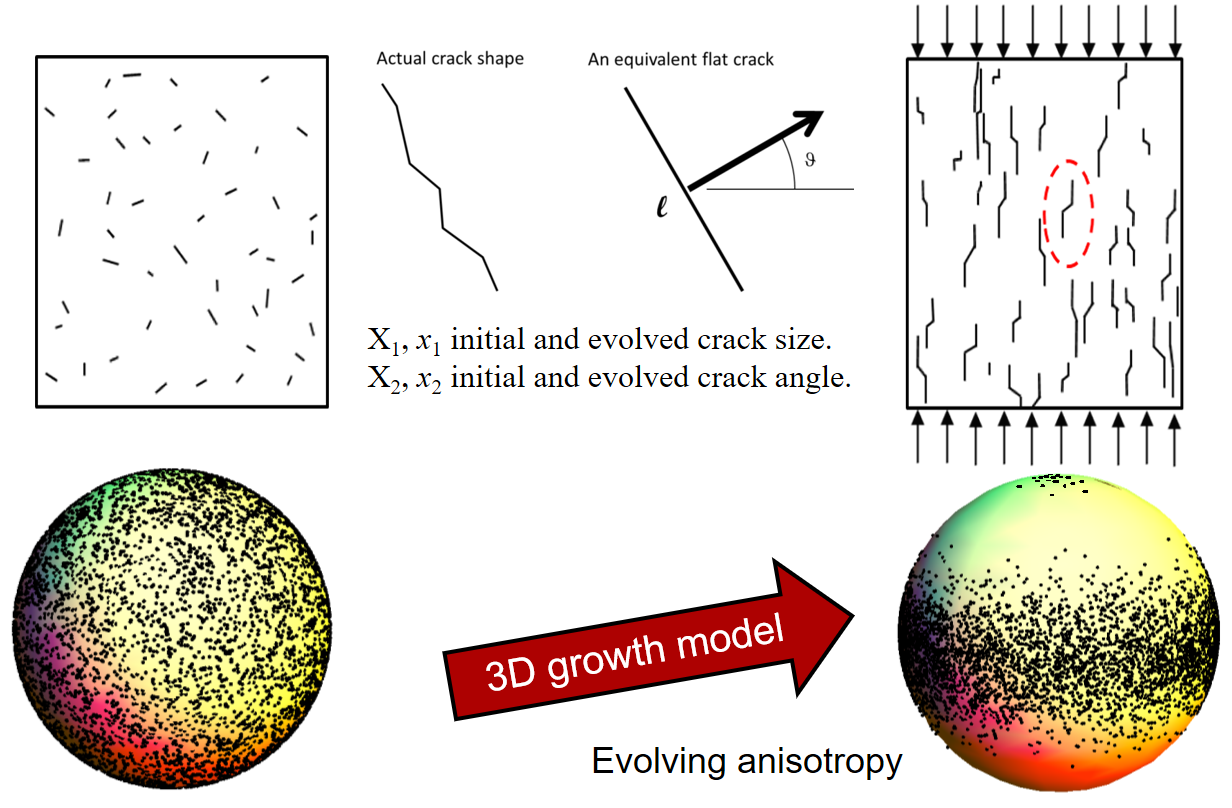
Abstract: Even if a ceramic’s homogenized properties (such as anisotropically evolving stiffness) truly can be predicted from complete knowledge of sub-continuum morphology (e.g., locations, sizes, shapes, orientations, and roughness of trillions of crystals, dislocations, impurities, pores, inclusions, and/or cracks), the necessary calculations are untenably hypervariate. Non-productive (almost derailing) debates over shortcomings of various first-principles ceramics theories are avoided in this work by discussing numerical coarsening in the context of a pedagogically appealing buckling foundation model that requires only sophomore-level understanding of springs, buckling hinges, dashpots, etc. Bypassing pre-requisites in constitutive modeling, this work aims to help students to understand the difference between damage and plasticity while also gaining experience in Monte-Carlo numerical optimization via scale-bridging that reduces memory and processor burden by orders of magnitude while accurately preserving aleatory (finite-finite-sampling) perturbations that are crucial to accurately predict bifurcations, such as ceramic fragmentation.
This publication helps to set knowledge needed to migrate cracks from initially uniform orientations (represented as dots on the left sphere) to highly textured orientations of vertical cracking (or any other texture based on the loading history).
This publication uses this simple system to explain many complicated concepts:

This paper would serve as a good project for a smart undergrad or first-year grad student to reproduce the results. It would serve as a familiarization exercise to learn basics of scale bridging, the difference between damage and plasticity, the influence of loading rate, the influence of microscale perturbations in macroscale behavior (e.g. reducing peak strength and scale effects), and binning down an excessively large number of internal variables to obtain a tractable decimated set. All of that without needing to know anything about constitutive modeling – just a basic knowledge of springs and rigid links would be needed.
Again: see it for free (until May 24) at
https://authors.elsevier.com/a/1WqS83PCJl7pmB
Python source code is available on request.
Cite the paper as:
Brannon, R., Jensen, K., and Nayak, D., Journal of the European Ceramic Society (2018), https://doi.org/10.1016/j.jeurceramsoc.2018.02.036
I plan to add this transformation to my upcoming book on computational geometry. This mapping was originally conceived to provide a one-to-one correspondence between RGB color and locations on a dance floor for a positioning correction in a project on robotic square dancers, but then we realized that simply laying down QR codes with coordinate and orientation data would be far more accurate.
 So what might be a good application for this transformation? It essentially maps the surface of the RGB cube (i.e., all fully saturated colors) to a square. One possibility would be to extend color plots that are conventionally used to depict one one variable to instead show two variables. In mechanics, for example, engineers typically show two different color plots for pressure and temperature, each with its own a linear legend bar ranging from a logical coordinate eta from 0 to 1, which is mapped to a selected linear color scheme (such as “hue” to range over the rainbow). In the single-variable color plots, the value of eta is set in proportion to the variable being plotted. To avoid needing two separate color plots for pressure and temperature a square color legend could be used with coordinates (eta1, eta2) associated with the two variables. While a “poor man’s” color plot mapping could be RGB[0,eta1,eta2], the one shown here would be far more spectacular because it would represent the full range of fully saturated colors (without “muddy” colors in the interior of the RGB cube) and, furthermore, values outside the range of interest would show as black.
I had some fun today mentoring a group of students to figure out how the wheels on their robot must be controlled in order to make it travel along a given Bezier curve (black line). We used animation to visually confirm our formulas.
Ed: This post shares an entertaining and insightful essay about customs, food, and women in Japan over 20 years ago. It was written by my friend and colleague, Mark Boslough, after he returned from an engineering business trip in Japan in 1994. I am curious how much has changed over the subsequent 20 years, so please comment if you know which of his observations or impressions no longer apply (or if they never applied in the first place too)! With Mark’s permission, this version has a few bits [in brackets] that have been altered to remove information that could identify particular individuals or organizations. It also has corrections of some minor typo/style issues. It is written in a style that mimics what Mark’s employer (a major US scientific research laboratory) required after any foreign travel.
CONTENTS:
Shown below is a scan of a piece of paper (with transcription) that I found in a file of my father’s old belongings. Even though this was about learning mathematics, it applies equally well to engineering. Any student who seriously follows tip number 7 will be an A student and, ultimately, a very productive and trustworthy engineer!

For now (to help with a conversation that I’m having with a few collaborators) this post provides only the following “infographic” to illustrate the concept of approximating a periodic discrete system with an effective continuum over a sufficiently large scale. (More information will be added about this topic as needed and/or as requested).
Below is shown a five-link chain (in red-blue-green-orange-black). Immediately this colorful chain is a dark-gray plot of the exact (mesocale) lineal density, which is defined at a location “x” to be the mass within an infinitesimal segment dx at that location divided by the segment’s length dx. This local density is shown as the dark-gray shaded plot in the upper-left corner, and it is the slope of the black line in the graph of the lower-left corner.
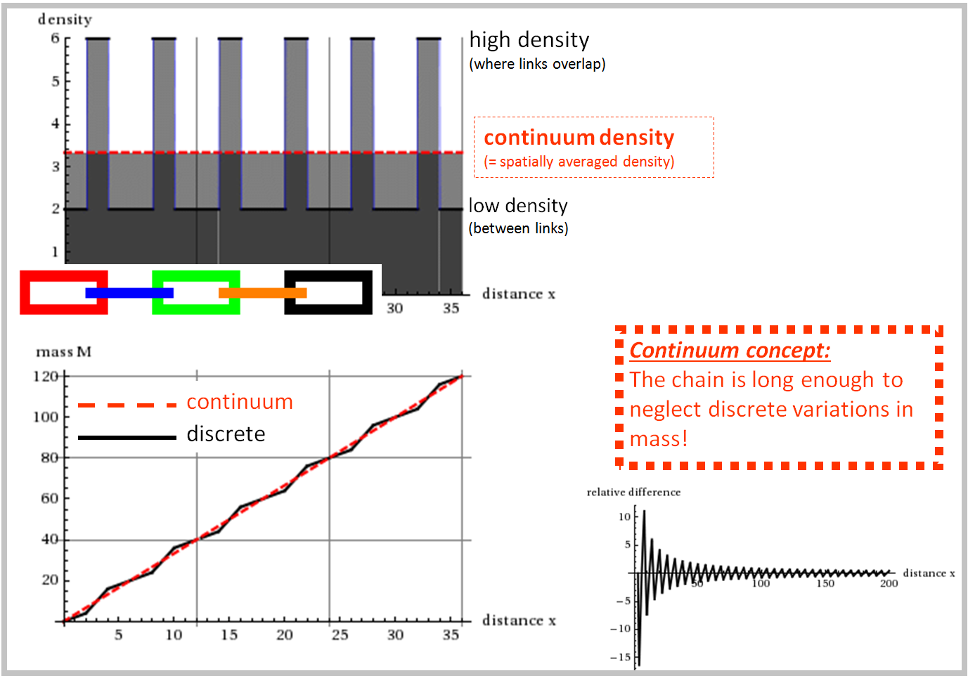
The continuum concept. Homogenization and identification of an RVE is based on the value of x for which perturbations fall below numerical round-off error for a given application.
The exact homogenized (macroscale) lineal density at a location “x” is defined as the exact total mass falling inside the span from zero to x, divided by the chain’s length (x itself). While the mesoscale density is the local slope at location “x” of the black line in the graph, the macroscale density is the secant slope at location “x” of the same black line. The continuum (red-dashed) approximation of the local mass distribution ignores local fluctuations from the fact that the chain is actually heterogeneous. For short chain lengths, the exact macroscale density is significantly different from the continuum density, but this discrepancy asymptotes toward zero as the chain length is increased.
The theoretical representative volume element (RVE) size corresponds to the size for which the discrepancy (like the plot in the lower-right corner of the infographic) falls below some tolerable threshold, which is determined by considering the tolerable error in an engineering simulation.
These concepts apply to other properties besides density. For example, the macroscale elastic stiffness would be defined as the force applied to the chain divided by the corresponding induced displacement. Like density, this macroscale property varies with the number of links in the chain, but it asymptotes to a steady value as the chain length increases.
Density has a nice asymptotic continuum limit that isn’t sensitive to dilutely distributed statistical perturbations in the local (microscopic) density. If, for example, 1 in 10000 links is made of light aluminum while the others are made of heavy steel, then the continuum density will be nevertheless close to that of a chain that is made entirely of steel links. The continuum elastic stiffness is likewise not highly sensitive to slight variations in local constituent (link) stiffness. A chain’s failure strength, on the other hand, is profoundly affected by existence of even a miniscule fraction of weaker links. A mostly steel chain that contains relatively few aluminum links would have a continuum strength equal to the strength of the weaker (aluminum) link. That’s because (in the limit) an infinitely long chain would contain at least one aluminum link. For short chains that are made of, say, 10 links (each of which has a 1 in 10000 chance of being made of aluminum), the average macroscale strength would be higher on average than the strength of longer chains. The strength data for short chains would also be more variable.
These observations give insight into what a modeler must pay attention to when using continuum macroscale properties in simulations of engineering structures. To design for the structure’s daily (i.e., normal and therefore usually elastic) usage conditions, homogenized continuum properties would be fine. However, continuum strength properties would need to be appropriately perturbed based on the size of the finite elements. This explicit incorporation of statistical variability in continuum properties is required when those perturbations strongly influence the engineering objective of the analysis (such as computing failure risk). In fact, it can be argued that such revisions are crucial to predict fracture and fragmentation whenever the finite-element size is smaller than a few kilometers. For more details on scale-dependent and statistically variable macroscale properties, see Publication: Aleatory quantile surfaces in damage mechanics and the more recent 2015 IJNME article, “Aleatory uncertainty and scale effects in computational damage models for failure and fragmentation” by Strack, Leavy and Brannon.
