I often get asked: when are you going to finish your tensor-analysis book?
Well, I have so many pressures on my time, that this hobby gets pushed to the bottom of the stack. This said, I find myself often discussing fourth-order tensor operations, the distinction between Voigt and Mandel components, and scalar measures of anisotropy. To help with such discussions, I am here posting two excerpts from my unpublished tensor-analysis notes. Enjoy this enthralling topic!
EDIT: you can now cite this topic from a real publication. It is in chapter 26 of my 2018 book: Rotation, Reflection, and Frame change.
The first excerpt from the still unpublished notes, 150606tensorsVoigtMandelExcerpt (for which the cited references may be found in 150606tensorsVoigtMandelExcerptReferences), discusses Voigt and Mandel notation, and introduces some helpful operations on fourth-order tensors. Here are some highlights taken from this PDF excerpt (all of which are included in the rotation book if you need to cite something):

What we have labeled as the 9×1 “contravariant Voigt array (without factors of 2)” is typically called a “stress-like” array in the composites community, while the 9×1 “covariant Voigt array (with factors of 2)” is called a “strain-like” array. When these arrays actually represent stress and strain, their last three entries are zero because of symmetry. Likewise, the 9×9 array is, in this context, the elastic stiffness so its last three columns and last three rows are zero because of minor symmetry. Accordingly, in constitutive modeling, you typically see this matrix relationship truncated down to only 6 dimensions. When using computer code to work out components of such tensors, we recommend keeping all 9 dimensions just to serve as a visual cue that you have indeed enforced symmetries properly in your equations.
It is mystifying that the composites community doesn’t seem to even realize that the Voigt representations would be more properly referred to as covariant and contravariant, so please add a comment to this post if you have ever seen any composites articles use this mathematically proper terminology. These are not just matrix equations. There is a tensor basis that goes with Voigt representations, and that basis is a set of mutually orthogonal tensors. The basis is not normalized, so that leads to co/contravariant representations, in which the factors of 2 are metrics. Whenever you have an orthogonal but not normalized basis, the obvious thing to do is to normalize it! That is what gives the following Mandel form, which you should note has no more of that ugly distinction between contravariant (stress-like) arrays and covariant (strain-like) arrays. Both arrays are treated the same!
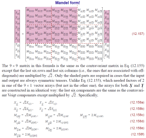
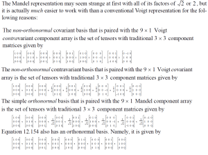
In this list, the very last set of basis tensors are the ones that pair with ordinary components of a tensor. For example, the 11 component of an ordinary second-order tensor is paired with a basis tensor whose component matrix is all zeros everywhere except a 1 in the 11 spot. The 12 component goes with a basis tensor that has all zeros everywhere except for a 1 in the 12 spot, and so on. The Voigt and Mandel representations merely represent a change of basis so that the first six basis tensors span the manifold of all possible symmetric tensors, while the last three basis tensors span the space of all possible skew tensors.
If you are not convinced that the Mandel representation is the better choice, try comparing it with Voigt for the components of the fourth-order identity tensor. The result is the identity matrix in Mandel form (not so for Voigt). Also, you really need the Mandel form to find eigenvalues and eigentensors. Ordinary spectral analysis of the Voigt representation is completely meaningless — you need to use Mandel form to get meaningful eigenvalues and eigenmodes of a stiffness tensor.
Page 658 (PDF page 30) of my second excerpt, 150606tensorsFourthOrderOperationsAndMeasureOfIsotropyExcerpt, shows how to find the isotropic (IFOET) part of a fourth-order tensor (which is NOT generally some multiple of the identity), and how to define a scalar measure of anisotropy in the range from zero to one, as determined from the “angle” that the tensor makes with the linear manifold of isotropic tensors. Doesn’t this sound exciting? Here is an infographic summary of this process of finding the isotropic part of a fourth-order tensor, as well as setting the scalar measure of anisotropy (equal to 1 minus the scalar measure of isotropy):
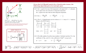
The isotropic part of a fourth-order tensor, as well as a scalar measure of anisotropy ranging from 0 to 1.
In this infographic, the acronym IFOET stands for “isotropic fourth-order engineering tensor” (labeled “ISO” elsewhere in the image). In the scalar measure of isotropy, the denominator is the L2 norm of the original fourth-order tensor, equal to the square root of the sum of the squares of the tensor’s Mandel components (which is another benefit of Mandel over Voigt because getting the magnitude of a Voigt tensor would require insertions of factors of 2 and 4 — Yuck!). As you can see, the isotropy is 100% if the original tensor is isotropic, and it ranges down to 0% isotropy if the isotropic part of the original tensor is zero.