Streamline visualization of tensor fields in solid mechanics

Stress net view of maximum shear lines inferred from molecular dynamics simulation of crack growth. Image from http://doi.ieeecomputersociety.org/10.1109/VIS.2005.33

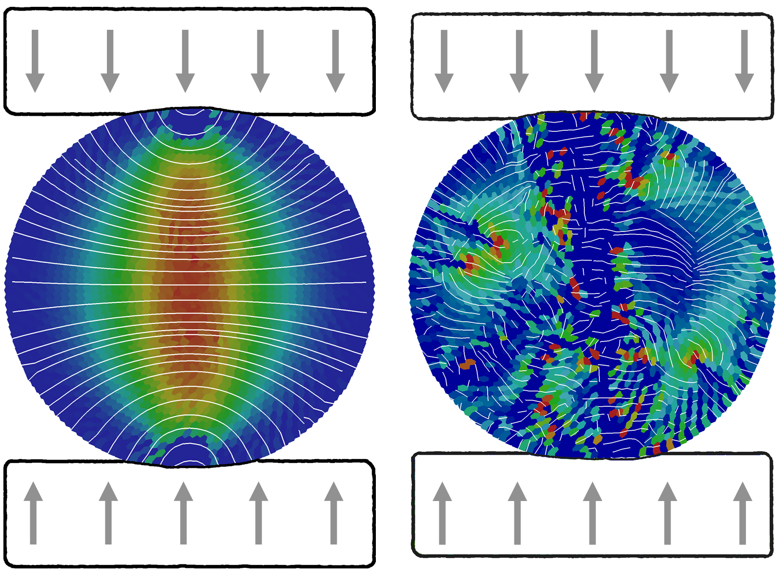
Brazilian stress net before and after material failure. Colors indicate maximum principal stress (showing tension in the center of this axially compressed disk). Lines show directions of max principal stress.

A stress net is simply a graphical depiction of principal stress directions (or other directions derived from them, such as rotating them by 45 degrees to get the maximum shear lines.)  Continue reading

Tutorial: Visualizing Deformation

If you’ve never heard of a continuum mapping, read our introduction to mappings.

This posting discusses the two most common visualization methods for 3D homogeneous mappings: Showing how a sphere transforms to an ellipsoid and how a cube transforms to a parallelepiped:
Sphere transforming to ellipsoidBox transforming to parallelepiped

Continue reading

Tutorial: multi-linear regression

The straight line is the linear regression of a function that takes scalars (x-values) as input and returns scalars (y-values) as output. (figure from GANFYD)

You’ve probably seen classical equations for linear regression, which is a procedure that finds the straight line that best fits a set of discrete points \{(x_1,y_1), (x_2,y_2),...,(x_N,y_N)\} . You might also be aware that similar formulas exist to find a straight line that is a best (least squares) fit to a continuous function y(x) .

The pink parallelogram is the multi-linear regression of a function that takes vectors (gray dots) as input and returns vectors (blue dots) as output

The bottom of this post provides a link to a tutorial on how to generalize the concept of linear regression to fit a function \vec{y}(\vec{x}) that takes a vector \vec{x} as input and produces a vector \vec{y} as output. In mechanics, the most common example of this type of function is a mapping function that describes material deformation: the input vector is the initial location of a point on a body, and the output vector is the deformed location of the same point. The image shows a collection of input vectors (initial positions, as grey dots) and a collection of output vectors (deformed locations as blue dots). The affine fit to these descrete data is the pink parallelogram. Continue reading

Publication: Decomposition and Visualization of Fourth-Order Elastic-Plastic Tensors

A.G. Neeman; R.M. Brannon; B. Jeremic; A. Van Gelderand;  A. Pang

Top view (Z from above) of eigentensors for Drucker-Prager material, time step 124, colored by minimum stretch eigenvalue.

Visualization of fourth-order tensors from solid mechanics has not been explored in depth previously. Challenges include the large number of components (3x3x3x3 for 3D), loss of major symmetry and loss of positive definiteness(with possibly zero or negative eigenvalues). This paper presents a decomposition of fourth-order tensors that facilitates their visualization and understanding. Fourth-order tensors are used to represent a solid’s stiffness.The stiffness tensor represents the relationship between increments of stress and increments of strain. Visualizing stiffness is important to understand the changing state of solids during plastification and failure. In this work,we present a method to reduce the number of stiffness components to second-order 3×3 tensors for visualization.The reduction is based on polar decomposition, followed by eigen-decomposition on the polar “stretch”. If any resulting eigenvalue is significantly lower than the others, the material has softened in that eigen-direction. The associated second-order eigentensor represents the mode of stress (such as compression, tension, shear, or some combination of these) to which the material becomes vulnerable. Thus we can visualize the physical meaning of plastification with techniques for visualizing second-order symmetric tensors.

Available Online:

Publication: http://www.mech.utah.edu/~brannon/pubs/7-2008NeemanBrannonJeremicVanGelderPang.pdf

Poster: http://www.mech.utah.edu/~brannon/pubs/7-09NeemanBrannonEtAlNEESposter.pdf