Transform between a cube’s surface and a square

I plan to add this transformation to my upcoming book on computational geometry. This mapping was originally conceived to provide a one-to-one correspondence between RGB color and locations on a dance floor for a positioning correction in a project on robotic square dancers, but then we realized that simply laying down QR codes with coordinate and orientation data would be far more accurate.

So what might be a good application for this transformation? It essentially maps the surface of the RGB cube (i.e., all fully saturated colors) to a square. One possibility would be to extend color plots that are conventionally used to depict one one variable to instead show two variables. In mechanics, for example, engineers typically show two different color plots for pressure and temperature, each with its own a linear legend bar ranging from a logical coordinate eta from 0 to 1, which is mapped to a selected linear color scheme (such as “hue” to range over the rainbow). In the single-variable color plots, the value of eta is set in proportion to the variable being plotted. To avoid needing two separate color plots for pressure and temperature a square color legend could be used with coordinates (eta1, eta2) associated with the two variables. While a “poor man’s” color plot mapping could be RGB[0,eta1,eta2], the one shown here would be far more spectacular because it would represent the full range of fully saturated colors (without “muddy” colors in the interior of the RGB cube) and, furthermore, values outside the range of interest would show as black.

Continuum homogenization and RVEs

For now (to help with a conversation that I’m having with a few collaborators) this post provides only the following “infographic” to illustrate the concept of approximating a periodic discrete system with an effective continuum over a sufficiently large scale. (More information will be added about this topic as needed and/or as requested).

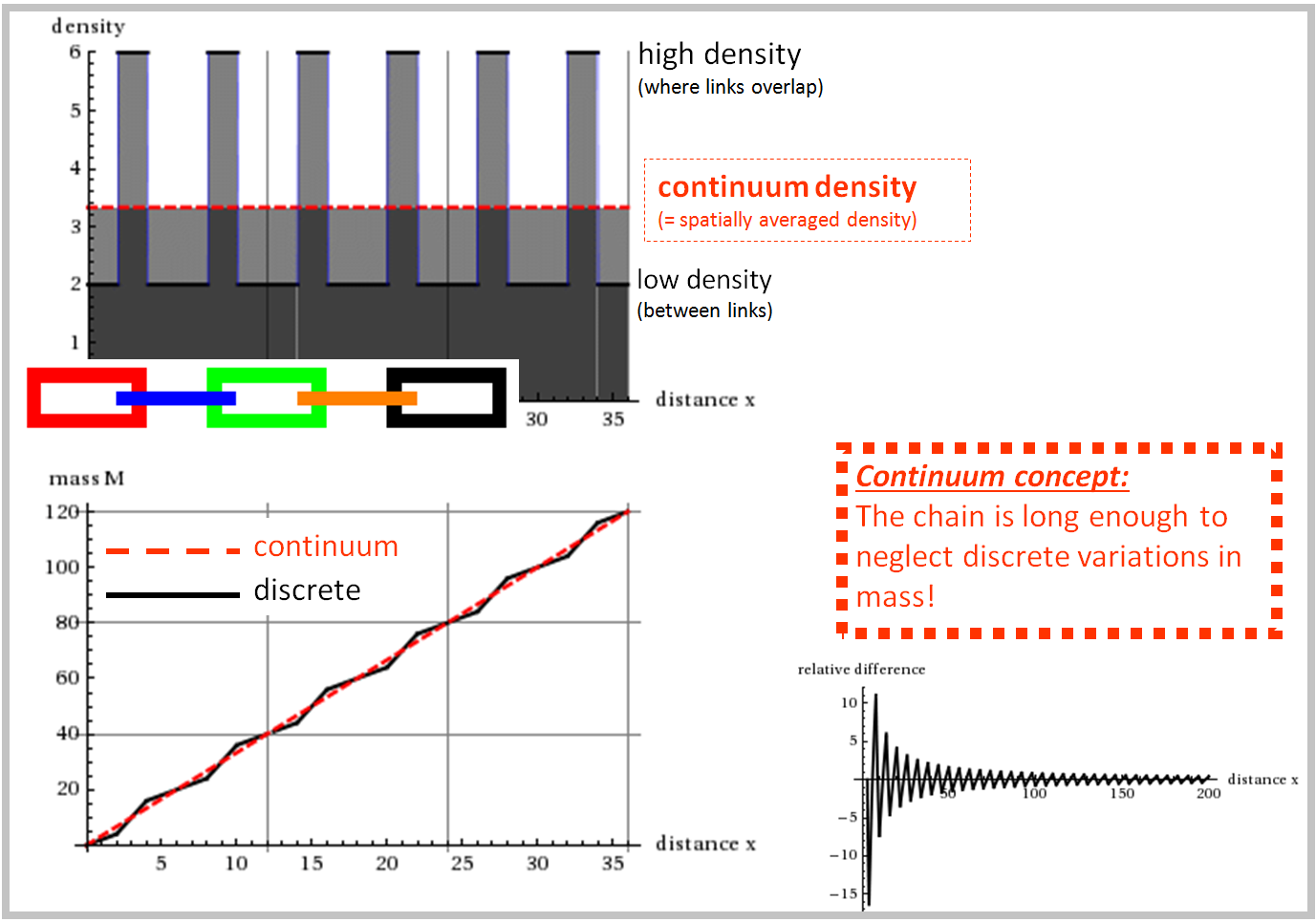
Below is shown a five-link chain (in red-blue-green-orange-black). Immediately this colorful chain is a dark-gray plot of the exact (mesocale) lineal density, which is defined at a location “x” to be the mass within an infinitesimal segment dx at that location divided by the segment’s length dx. This local density is shown as the dark-gray shaded plot in the upper-left corner, and it is the slope of the black line in the graph of the lower-left corner.

The continuum concept. Homogenization and identification of an RVE is based on the value of x for which perturbations fall below numerical round-off error for a given application.

The continuum concept. Homogenization and identification of an RVE is based on the value of x for which perturbations fall below numerical round-off error for a given application.

The exact homogenized (macroscale) lineal density at a location “x” is defined as the exact total mass falling inside the span from zero to x,  divided by the chain’s length (x itself).  While the mesoscale density is the local slope at location “x” of the black line in the graph, the macroscale density is the secant slope at location “x” of the same black line.   The continuum (red-dashed) approximation of the local mass distribution ignores local fluctuations from the fact that the chain is actually heterogeneous. For short chain lengths, the exact macroscale density is significantly different from the continuum density, but this discrepancy asymptotes toward zero as the chain length is increased.


The theoretical representative volume element (RVE) size corresponds to the size for which the discrepancy (like the plot in the lower-right corner of the infographic) falls below some tolerable threshold, which is determined by considering the tolerable error in an engineering simulation.

These concepts apply to other properties besides density. For example, the macroscale elastic stiffness would be defined as the force applied to the chain divided by the corresponding induced displacement. Like density, this macroscale property varies with the number of links in the chain, but it asymptotes to a steady value as the chain length increases.

Density has a nice asymptotic continuum limit that isn’t sensitive to dilutely distributed statistical perturbations in the local (microscopic) density.  If, for example, 1 in 10000 links is made of light aluminum while the others are made of heavy steel, then the continuum density will be nevertheless close to that of a chain that is made entirely of steel links. The continuum elastic stiffness is likewise not highly sensitive to slight variations in local constituent (link) stiffness.  A chain’s failure strength, on the other hand, is profoundly affected by existence of even a miniscule fraction of weaker links. A mostly steel chain that contains relatively few aluminum links would have a continuum strength equal to the strength of the weaker (aluminum) link. That’s because (in the limit) an infinitely long chain would contain at least one aluminum link. For short chains that are made of, say, 10 links (each of which has a 1 in 10000 chance of being made of aluminum), the average macroscale strength would be higher on average than the strength of longer chains. The strength data for short chains would also be more variable.

These observations give insight into what a modeler must pay attention to when using continuum macroscale properties in simulations of engineering structures.  To design for the structure’s daily (i.e., normal and therefore usually elastic) usage conditions, homogenized continuum properties would be fine. However, continuum strength properties would need to be appropriately perturbed based on the size of the finite elements. This explicit incorporation of statistical variability in continuum properties is required when those perturbations strongly influence the engineering objective of the analysis (such as computing failure risk). In fact, it can be argued that such revisions are crucial to predict fracture and fragmentation whenever the finite-element size is smaller than a few kilometers. For more details on scale-dependent and statistically variable macroscale properties, see Publication: Aleatory quantile surfaces in damage mechanics and the more recent 2015 IJNME article, “Aleatory uncertainty and scale effects in computational damage models for failure and fragmentation” by Strack, Leavy and Brannon.

Undergraduate researcher applies binning to study aleatory uncertainty in nonlinear buckling foundation models

20150721_KatharinJensenAvatar

Sophomore undergraduate, Katharin Jensen, has developed an easily understood illustration of the effect of aleatory uncertainty, which means natural point-to-point variability in systems. She has put statistical variability on the lengths of buckling elements in the following system:

bistableSystem

Continue reading

Errata for two verification publications

computer-doh

This posting provides errata for an analytical solution that appeared in the following two publications:

Brannon, R. M. and S. Leelavanichkul (2010) A multi-stage return algorithm for solving the classical damage component of constitutive models for rocks, ceramics, and other rock-like media. Int. J. Fracture v. 163(1), pp. 133-149.

K.C. Kamojjala, R. Brannon, A. Sadeghirad, and J. Guilkey (2013) Verification tests in solid mechanics, Engineering with Computers, 1-21.

As pointed out by Dr. Andy Tonge, they both contain a the same transcription error that was not in the original unpublished working document where the details of the solution are archived.  The following excerpt from the original unpublished working document contains correct formulas:  PlasticityVerification2excerpt.   See the red comment boxes in this file for details.

Streamlines, Streaklines, Pathlines, and Gridlines

GridStreamStreakPath

The above animation aims to be a slight improvement over one on Wikipedia, which (incidentally) does not correctly describe the velocity field that it is depicting. The Wikipedia image doesn’t show a checkerboard of moving material, nor does it have a nice depiction of streamlines.

Before describing this animation, it might be helpful to look at a simpler motion (a rolling body) in order to review the difference between streamlines, streaklines, and pathlines. Consider a simple rigid body consisting of a disk of small radius (shown in gray below) along which it rolls along a tabletop, along with a larger-radius extension of the body (shown in color below) which can dip down below the table surface (as if there is a slot cut into the table so that part of the body rolls under it).

STREAMLINES: These are tangent to the instantaneous velocity field.  For a rolling rigid body, the motion is always circular about the instantaneous center of rotation at the bottom of the wheel. Accordingly, this image shows the streamlines at various points in time as the disk rolls along:

particleStreamLineRolling

This image of streamlines is drawn not just on the body itself but also on its “virtual extension” in order to emphasize that (for rigid rolling) the instantaneous velocity is circular around the instantaneous center of rotation (bottom of the wheel). A particular set of streamlines is drawn in red. These are the ones that pass through a set of points that are evenly distributed on a spoke of the wheel (shown in black).

STREAKLINES: These are the lines you would see if a magic gremlin were to sit at a given location in space and “spraypaint” the material as it passes by.  Suppose that an assembly line of gremlins (located where you see the dots in the first image) are pointing their spray paint cans at the body while it rolls past. Then they would form the black streaklines shown here at various times:

streaklinesOnBefore

Important: The streaklines are made by gremlins who are sitting still and spraying material as it passes by.

PATHLINES: Are made by gremlins who “ride” with the material, spraying a record of where they have been (as if we were watching the rolling body from behind a window, and those whacky gremlins would spray paint onto the window as they pass by). Accordingly, here are the pathlines for group of gremlins who were initially coincident with the gremlins in the above streakline plot:

particlePathLineRolling

GRIDLINES are any set of lines that are painted on the body like tattoos. Such lines move with the body (like a tattoo).


Continue reading

Publication: Verification tests in solid mechanics

ABSTRACT: Code verification against analytical solutions is a prerequisite to code validation against experimental data. Though solid-mechanics codes have established basic verification standards such as patch tests and convergence tests, few (if any) similar standards exist for testing solid-mechanics constitutive models under nontrivial massive deformations. Increasingly complicated verification tests for solid mechanics are presented, starting with simple patch tests of frame-indifference and traction boundary conditions under affine deformations, followed by two large-deformation problems that might serve as standardized verification tests suitable to quantify accuracy, robustness, and convergence of momentum solvers used in solid-mechanics codes. These problems use an accepted standard of verification testing, the method of manufactured solutions (MMS), which is rarely applied in solid mechanics. Body forces inducing a specified deformation are found analytically by treating the constitutive model abstractly, with a specific model introduced only at the last step in examples. One nonaffine MMS problem subjects the momentum solver and constitutive model to large shears comparable to those in penetration, while ensuring natural boundary conditions to accommodate codes lacking support for applied tractions. Two additional MMS problems, one affine and one nonaffine, include nontrivial traction boundary conditions.

For a copy of the paper along an implementation of the vortex problem, see our simple matlab MPM code.

Here are some eye-catching graphics (see the paper itself for details):

2013verificationPic1 Continue reading

Holey Particle Basis functions for 2D CPDI

allpictab

An older post (https://csmbrannon.net/2013/09/29/particle-basis-function-in-the-cpdi-method/) showed particle basis functions in 1D, demonstrating that they retain overlapping support with neighboring particles when using CPDI even when the particles are stretched to be large multiples of the grid cell length. In the 1D context of those examples, “holes” in CPDI basis functions are impossible.

This post shows an extreme 2D example (suggested by John Nairn, Jim Guilkey, and Michael Homel*) that can deleteriously lose overlapping support of particle shape functions, which can then allow non-physical material interpenetration.

Continue reading

Uintah Simulations of Perforation Experiments

Perforation

ABSTRACT: A simulation of a simple penetration experiment is performed using Material Point Method (MPM) through the Uintah Computational Framework (UCF) and interpreted using the post-processing visualization program VisIt. MPM formatting sets a background mesh with explicit boundaries and monitors the interaction of particles within that mesh to predict the varying movements and orientations of a material in response to loads. The modeled experiment compares the effects of an aluminum sphere impacting an aluminum sheet at varying velocities. In this work, the experiment called launch T-1428 (by Piekutowski and Poorman) is simulated using UCF and VisIt. The two materials in the experiment are both simulated using a hypoelastic-plastic model. Varying grid resolutions were used to verify the convergent behavior of the simulations to the experimental results. The validity of the simulation is quantified by comparing perforation hole diameter. A full 3-D simulation followed and was also compared to experimental results. Results and issues in both 2-D and 3-D simulation efforts are discussed. Both the axisymmetric and 3-D simulation results provided very good data with clear convergent behavior.

See the link below for the full report.

Experiment in Uintah

Continue reading