Sophomore undergraduate, Katharin Jensen, has developed an easily understood illustration of the effect of aleatory uncertainty, which means natural point-to-point variability in systems. She has put statistical variability on the lengths of buckling elements in the following system:

Each of the buckling hinges has a lateral spring support (not shown above, but illustrated below) which resists axial loads up to a buckling limit. This system was chosen because it is typically the first example of a buckling system seen by undergraduates, and our goal for this work is to illustrate the profound effect of aleatory uncertainty (i.e., irreducible statistical variability in micromorphology such as link lengths) in a context that any undergraduate student of mechanics can understand. The trends shown here (especially when Katharin’s code is revised to allow damage in the form of broken lateral support springs) are similar to what we see in failure data for ceramics.

In the above plot, the red dashed line shows the force-displacement response of this 5-element system in the absence of any variability in buckling component lengths. The dark line illustrates that including variability in the buckling component lengths produces a reduction in the overall strength (peak force). This system is 100% elastic and recoverable, meaning that the force-displacement plot is retraced backward if the plate is pulled upward after any degree of compression.  In addition to illustrating the effect of geometric variability, this system therefore also debunks the myth that reaching a peak in a force-displacement plot indicates material damage — there is no damage in this plot!  This system is displacement controlled, and hence it is stable even after the peak.   The fact that the peak force with variability is smaller than that of the idealized perfect system also gives you a hint about why Euler buckling theory is not conservative: it fails to account for natural perturbations in the material that stimulate premature instability.

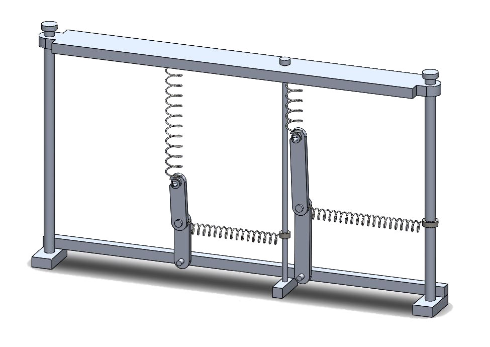
A two-element system drawn in 3D to clarify the equations being solved. Each buckling component has a horizontal supporting spring on a slider.

QUESTIONS: When the component geometry is allowed to vary statistically, how much change is expected in the force-displacement plot? Is there a dependence on the number of elements in the system? The 3D image (at left) shows two elements in parallel (each element is a spring and buckling component in series). The opening animation showed a five-element system.  The family of graphs below depicts the expected variation in force-displacement plots of a 10-element system. Each blue line is the force-displacement plot for a 10-element realization of statistically variable link lengths.

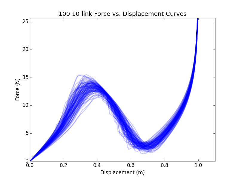
As the number of elements is increased, the simulations take a long time to run. Katharin was able, however, to use the binning scheme at https://csmbrannon.net/2015/07/20/publication-binning/ to reduce her calculation run time from 1 hour down to only 7 seconds!

For all the gory details of this work on probabilistic foundation modeling, please see the fifty-page report:
Buckling Link and Spring System
(written entirely by sophomore undergraduate investigator, Katharin Jensen)

Here is a dropbox link to Open-source python code. (for access to the github repo, please send a request to katharin.jensen@utah.edu)

Below are a few more of Katharin’s movies.

1. The first one is a 100% elastic system showing retracing of the path upon displacement reversal and hence no dissipative hysteresis (this simulation, BTW, debunks the remarkably persistent myth that reaching a peak in a force-displacement plot is necessarily a sign of irreversible damage or plasticity — this system is perfectly elastic).  The springs are nonlinearly elastic to ensure that it takes infinite force to compress a spring to zero length — that’s why the plot has an upward curvature in the pre-buckling zones.
   
2. The 2nd simulation shows effects of damage, where you see hysteresis caused by irreversible changes in the system stiffness without permanent (plastic) displacement. This effect is modeled by allowing the lateral support spring to “break” after a critical amount of deformation. Again, the key feature is that there is hysteresis but no residual deformation after removal of the load.  Hysteresis means that the deformation is inelastic, and the fact that the response goes back to the origin is a sign that the inelasticity merely causes a reduction in elastic stiffness. Also note that partial damage is possible as a direct result of aleatory uncertainty (the deterministic red-dashed line drops to zero stress and zero stiffness instantaneously).
   
3. The 3rd simulation models friction in the lateral support (like a spring and sliding element in series), which is similar to plasticity where you see residual displacement upon removal of load.
   
4. The 4th simulation shows time-dependent phenomena by including mass for inertia and also by introducing viscosity from a dashpot in the lateral supports for the buckling elements.
   

It is the raw simplicity of these systems that is appealing for educating students about the general effects of microstructure on macroscale response, as well as the profound influence of statistical variability in geometry.

Don’t forget: these were done by a sophomore (Katharin Jensen) after she took a first course in statics, dynamics, and numerical methods. Awesome!   Katharin is ultimately interested in mechatronics. Given her success in this project, we hope that she will consider research in flexible robots.