The following Material Point Method (MPM) simulation of sloshing fluid goes “haywire” at the end, just when things are starting to settle down:

(if the animated gif isn’t visible, please wait for it to load)

The following Material Point Method (MPM) simulation of sloshing fluid goes “haywire” at the end, just when things are starting to settle down:
(if the animated gif isn’t visible, please wait for it to load)

Motion without superimposed rotation
Same deformation with superimposed rotation
When developing constitutive models, it is crucial to run the model under a variety of standard (and some nonstandard) homogeneous deformations. To do this, you must first describe the motion mathematically. As indicated in http://csm.mech.utah.edu/content/wp-content/uploads/2011/03/GoBagDeformation.pdf, a good way to do that is to give the deformation gradient tensor, F. The component matrix [F] contains the deformed edge vectors of an initially unit cube, making this a very easy to way to prescribe deformations.
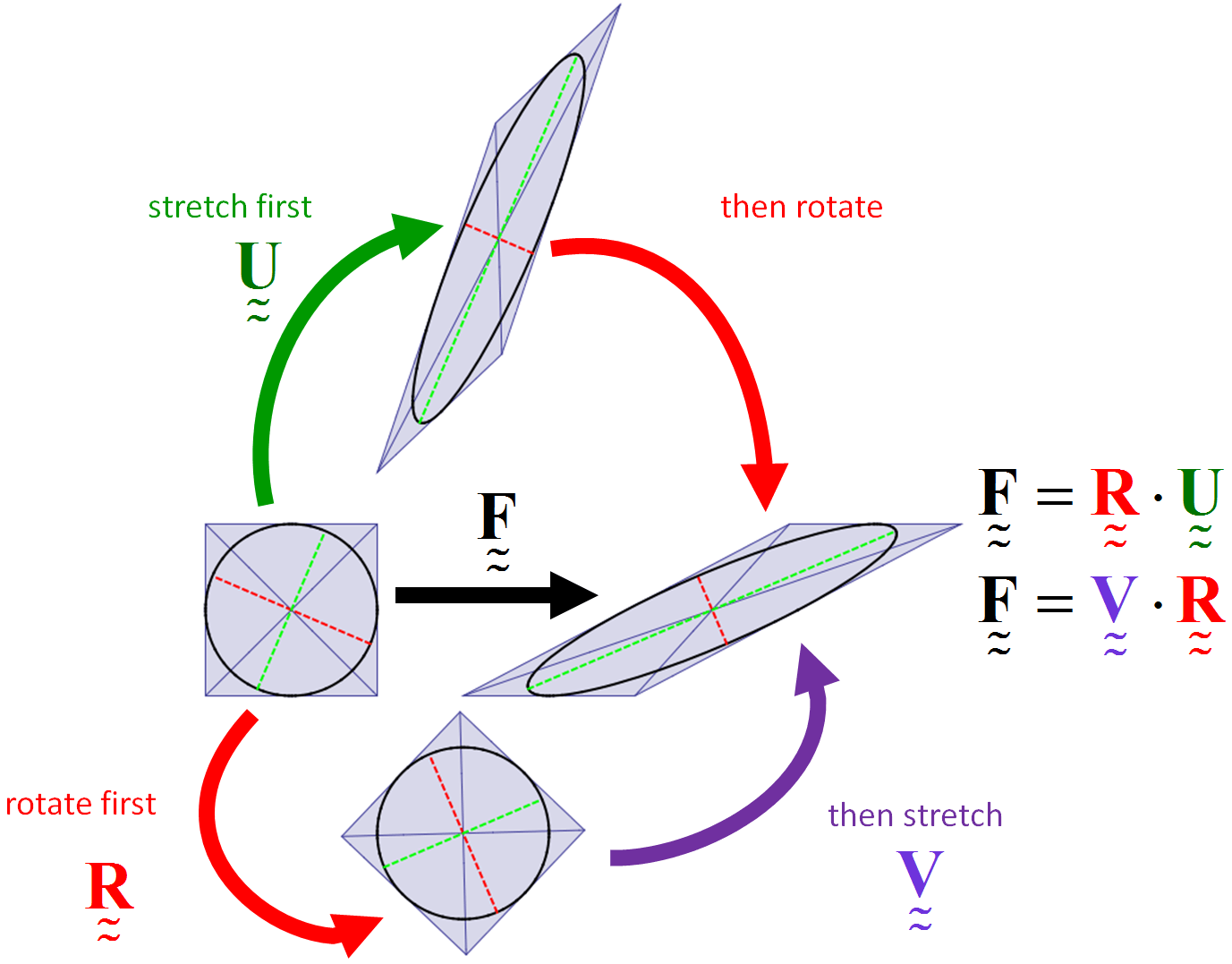
This posting explains the meaning of a polar decomposition, and it gives two numerical methods for computing it.
Below is shown simple shear of a unit square. The inscribed circle and the lines from corner to corner should be regarded as painted on the material, so they flow with deformation. The green and red dashed lines show the principal directions of stretch, which are aligned with the major axes of the deformed ellipse and hence move relative to the material as the deformation proceeds. In the deformed state (far right), the red and green dashed lines are defined to be aligned with the major axes of the deformed ellipse (far right). The red and green dashed lines in the other states show the material points covered by those green and red lines in the deformed state.
The animation below shows
RED: simple shear in physical configuration
BLUE: simple shear with the polar rotation removed (i.e., the pure stretch)
GREEN: the deformation corresponding to the approximation that D-bar (given by the unrotated symmetric part of the velocity gradient) is actually the rate of reference logarithmic strain. This is found by integrating D-bar through time to obtain the apparent logarithmic strain, and then exponentiating this apparent strain to obtain an apparent reference stretch.
GRAY: rotation of the green deformation back to the spatial configuration.

Illustrated below is the solution to an idealized problem of a linear elastic annulus (blue) subjected to twisting motion caused by rotating the T-bar an angle 
This simple problem is taken to be governed by the equations of equilibrium 
The logarithmic (Hencky) strain is evaluated by taking the log of the symmetric stretch tensor in continuum mechanics. Doing so requires transforming to the principal stretch basis, taking logs of the principal stretch eigenvalues, and transforming the result back to the lab basis. While this procedure is a bit tedious, it certainly is straightforward.
 The harder — almost freakishly daunting — question is: how do you get the rate of the logarithmic strain? This rate must include contributions from both the rate of the stretch eigenvalues and the rate of the stretch eigenvectors, which is difficult to handle when there are repeated eigenvalues causing extra ambiguity of eigenvectors. Continue reading
