This posting explains the meaning of a polar decomposition, and it gives two numerical methods for computing it.

Below is shown simple shear of a unit square.  The inscribed circle and the lines from corner to corner should be regarded as painted on the material, so they flow with deformation.  The green and red dashed lines show the principal directions of stretch, which are aligned with the major axes of the deformed ellipse and hence move relative to the material as the deformation proceeds.  In the deformed state (far right), the red and green dashed lines are defined to be aligned with the major axes of the deformed ellipse (far right). The red and green dashed lines in the other states show the material points covered by those green and red lines in the deformed state.

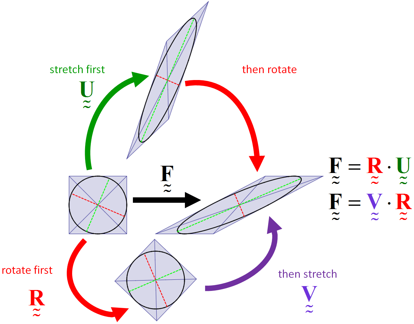
In the “rotate first” decomposition , the material is rotated (bottom figure) and then stretch is applied along the green and red dashed lines to end up in the final configuration. In the “rotate last” decomposition $latex \mathbf{F}=\mathbf{R}\cdot\mathbf{U} $, the material is stretched along the green and red dashed lines (top figure) and then rotated into place to end up in the final configuration.

The following animation better illustrates that principal stretch directions (red and green dashed lines defining the major axes of the ellipse) do not flow with the material:

In this animation, black lines (and curves) are material lines, which means they are “painted” on the material and hence flow with the material.  The top image shows what the deformation would look like if the deformation’s polar rotation is removed so that the red and green lines remain of the same orientation in both the top and far-left image.  The bottom image shows what the deformation would look like if stretching were removed so that only overall rigid rotation is shown. You should be able to infer from this animation that the rotation angle will approach 90 degrees; there is not an infinite amount of material rotation in conditions of simple shear (and that’s why the vorticity is NOT a measure of material rotation — to get material rotation, you need the spin associated with the polar rotation tensor).

Keep in mind: black lines are painted on the material. The red and green lines, however, are NOT material lines, so think of them as being highlighted by someone holding red and green laser pointers to illuminate ever-changing locations of interest. The red and green lines in the far right (deformed) configuration show the major axes of the deformed ellipse. You can’t locate the red and green lines in the far-left (undeformed) image until you first locate them in the far-right (deformed) image.  In the far-left (undeformed) image, the red and green lines are so-called “pre-images” of the ones in the right image. In other words, they are drawn over the original locations of the material points that are currently underneath the principal axes of the deformed ellipse.

As seen, the red and green lines in the far left image are not stationary. That means different material fibers suffer the biggest (or smallest) stretching depending on how far along the deformation has gone. Initially, for example, the green line is angled at 45 degrees, so material fibers with that orientation are elongated more than any other fibers.  The situation changes as deformation proceeds.   With increasing shear, the green line in the initial configuration (far left image) rotates counter-clockwise towards a vertical orientation (in the left-side image). Meanwhile, the green line in the far-right (deformed) configuration rotates clockwise towards the horizontal to stay always oriented with the largest ellipse axis. This means that initially vertical (not angled) lines ultimately will be the ones that suffer the most elongation under shear; these lines (once stretched under the action of shearing) will be will be ultimately aligned with the horizontal direction in their deformed state.

 

---

Higham numerical method (for 3×3 polar decomposition).
The following fixed-point algorithm repeatedly averages a 3×3 matrix with its own inverse-transpose. Doing this over and over again will make the matrix converge to the polar rotation as long as the starting matrix has a positive determinant. Alert: there does exist an exact analytical solution for the 3×3 polar decomposition (cf. Simo and Hughes), but it is not only less efficient — it’s also less accurate! Reason: The analytical solution requires trigonometric functions, which are both expensive and have higher round-off errors than iterative solvers.

Step 1a: read in the 3×3 matrix (and, optionally for SQA, include a sanity check to confirm that the determinant of the matrix is positive).

Step 1b: Initialize a “helper” matrix:

Step 2: Compute an updated approximation for the polar rotation to be the average of with its own inverse-transpose:

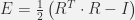
Step 3: Compute the error (strain) matrix
.
Set an overall scalar error to be the norm,

Step 4: If , where “TOL” is a small tolerance, then set and go to step 2; otherwise, the algorithm has converged to the polar rotation, so continue to STEP 5.

Step 5: Compute the stretch matrices:

and

Step 6: Perform optional SQA checks:

• Confirm that and  are symmetric
• Confirm that and  are positive definite!
• Confirm that the matrices
  
  and
  
  are each acceptably close to zero.

 

COMMENT: In Steps 1 and 6, “SQA” stands for “software quality assurance.” You should include SQA in your source code until the algorithm is extensively tested.  The test for positive definiteness of the stretches is crucial. It is remarkable how many polar-decomposition routines are out there that only test for symmetry and hence incorrectly identify the matrix

as a stretch merely because it is symmetric. This is a 180 degree rotation (for which the stretch is the identity matrix)!  In fact, the matrix will be symmetric, yet not a stretch if and only if the rotation angle is exactly 180 degrees. Accordingly, it is important to test this special case in any polar decomposition software.

COMMENT: In Step 3, if is the polar rotation, then it will be orthogonal, making the error (strain) matrix zero. Warning: do not use an -norm to check if the matrix is sufficiently close to zero. While the -norm is indisputably efficient, it does not transform as a proper tensor-to-scalar operation under a change of basis and could therefore result in your code giving different answers at different angles in applications (a symptom might be a drift of answers at 45 degrees relative to those at 0 and 90 degrees in a problem that is supposed to be axisymmetric). The norm suggested in Step 3, on the other hand, will ensure that the number of iterations is insensitive to the observer orientation (i.e., the local basis to which components are referenced).

COMMENT: In Step 4, a good choice for the tolerance value is . If you wish to make your software accurate to machine precision, don’t use a tolerance. Instead, simply continue iterations until adding the error to the numeral 1.0 results in 1.0. That is,
“do while” .

---

Super fast analytical (and numerical) method for 2×2 polar decomposition
There is a wonderful — and surprisingly little-known — method to get a polar decomposition for a 2×2 matrix

Step 1: Compute two helper numbers:

and

Step 2: Compute the cosine (c) and sine (c) of the rotation angle:

and

Step 3: Construct the polar rotation matrix:

Step 4: If desired, obtain stretches as was done in the Higham algorithm.

COMMENT: This method is so cool.  Try using it to obtain the polar rotation for the simple shear motion used in this posting’s animations, and then compare how trivially easy it is in comparison to the traditional method (which gets stretch first via solving an eigenproblem)!

COMMENT: The above algorithm also generalizes easily to any 3×3 matrix that is of “planar” form.