These images show the initial configuration of a body (square) and a nonlinear deformation of that body into a curvy shape (to the right of the square).  Overlaid on the actual deformed shape is the so-called tangent mapping at the indicated point.  It coincides with the nonlinear mapping to first-order accuracy.

Background

Grade school children (or college freshman in some countries) learn that any nonlinear function has a local tangent mapping at any point of interest, , which is simply the straight-line tangent to the nonlinear curve at that point.  The equation of the tangent mapping in this case is

, where evaluated at and .

Analogously, consider the nonlinear “material mapping” transformation commonly studied in continuum mechanics:

Input:  Initial position vector of a point  in the body

Output: Deformed position vector  of the same point.

The “output” (deformed location of a point)  is generally nonlinearly related to the “input” (initial location of a point), which is why the initial square in the animations deforms to a curvy shape. However, just as the nonlinear function has a local straight-line tangent line, this vector-to-vector transform also has a tangent mapping.  The tangent mapping at a point in the initial configuration of the body (red dot in the animations) is defined by

,

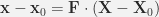
where

is the deformation gradient tensor having components

is the deformed location of the point initially located at (blue dot in the animations)

Evidently, the deformation gradient tensor plays a role similar to the role played by slope ““ in the scalar case of .