Illustrated below is the solution to an idealized problem of a linear elastic annulus (blue) subjected to twisting motion caused by rotating the T-bar an angle .  The motion is presumed to be applied slowly enough that equilibrium is satisfied.

This simple problem is taken to be governed by the equations of equilibrium , along with the plane strain version of Hooke’s law in which Cauchy stress is taken to be linear with respect to the small strain tensor (symmetric part of the displacement gradient).  If this system of governing equations is implemented in a code, the code will give you an answer, but it is up to you to decide if that answer is a reasonable approximation to reality. This observation helps to illustrate the distinction between verification (i.e., evidence that the equations are solved correctly) and validation (evidence that physically applicable and physically appropriate equations are being solved).  The governing equations always have a correct answer (verification), but that answer might not be very predictive of reality (validation).

In what follows, r, , and z are the cylindrical coordinates of the initial position vector. The stated governing equations are almost certainly invalid under large deformations (where both geometric and material nonlinearity are important). Nevertheless, because the stated equations still have a solution when applied under large twist angles, it is still a good idea to run verification tests of your small-deformation code in the large deformation context.  Just don’t kid yourself into believing the answer is realistic.

The exact solution to the stated governing equations is summarized as follows: Assuming an isotropic material, the symmetry of the problem implies that out-of-plane shear stress components  must be zero and all other stress components with respect to the cylindrical basis must depend exclusively on the radial coordinate r. In this case, the equations of equilibrium,

reduce to

(1)    

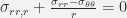
(2)    

Here, comma denotes differentiation. These are now ordinary differential equations because symmetry reduces the number of independent variables down to only the radial coordinate r. Since the second equilibrium equilibrium equation (2) is a an ordinary differential equation that has only one dependent variable, , you can solve it immediately without any need to introduce a constitutive model.  To set the integration constant to a physically meaningful value, you can require that the net torque on the rod be given by some known value T.  Following through shows that the shear stress depends on the radial coordinate r, the height of the annulus H, and the net torque T according to

(3)    

The fact that this result holds for any choice of constitutive model can be confirmed using the much more elementary approach of analyzing moment balance for the free body diagram of material falling within the radius r.  Finding the other stress components, and finding the relationship between the torque and material motion, requires using the constitutive model.

From axisymmetry, note that the polar components of displacement, and depend only on the radial coordinate r. You must not, however, assume that the radial component of displacement is zero.  Even if you were to assume purely circular motion, making the radius constant, there would still be a nonzero radial component of displacement; this fact is used later to set the boundary conditions for the displacement field.  As seen in the above image, the exact solution to the governing equations exhibits radial motion anyway, so both components of displacement must be allowed to be nonzero if you wish for this analytical solution to be used in verification testing of a code. Since both the radial and circumferential displacement components depend only on  r, the small strain tensor (= symmetric part of the displacement gradient) reduces to

(4)    

(5)    

(6)    

Substituting these strain components into Hooke’s law gives the stress as a differential function of the displacement field. Substituting the resulting stress components into the equilibrium equations leads to ordinary differential equations for the two displacement components.  Of course, to solve them, we need boundary conditions. Let a and b denote the inner and outer radii of the deforming (blue) material.  As indicated in the animation, the outer ring at is stationary, giving

(7a)

(7b)

Let denote the twist angle of the rod (i.e., the angle between the solid and dashed lines in the figure). Shown below is an arc representing the purely circular motion of any point on the inner rod from an initial position X to final position x. To match the twist angle at , the final solution for the displacement field must have the property that any position vector on the surface of the rod must rotate by an angle .  The first step is to use the image below to find the components of the initial and current position vector with respect to the reference cylindrical base vectors:

Then resolving the displacement vector, u=x–X, into radial and tangential parts implies the following additional boundary conditions:

(8a)    

(8b)    

You should be now questioning our choice of cylindrical base vectors.  Does it make sense that we used the reference cylindrical basis (the one aligned with X)?   Below we discuss the possibility that perhaps we should have used the current cylindrical basis rather than the reference basis; that discussion reinforces the difference between verification and validation. By writing Eq. (8), we are providing a clear statement of the differential equation being solved (since specification of boundary conditions is part of a complete specification of a boundary value problem). Thus, our equations are well posed and should therefore be solved correctly (verification) even if they are not the physically appropriate equations to be solved (validation).   For now, let’s accept the equations as written and proceed with stating the solution. Enforcing the boundary conditions in (7) and (8) leads to the following finalized results for the displacement field:

(9)    

(10)   

This implies that a point with initial Cartesian components

(11)   

(12)  

will deform to a new position with Cartesian components

(13)  

(14)  

The deformed position vector of any other point on the annulus may be found by applying a rotation to this solution, where the rotation angle is the polar coordinate angle of the initial particle location. Interestingly, note that the solution for the deformed position is independent of the elastic properties, but that doesn’t mean that the solution is independent of the constitutive model.  It is the linearity of Hooke’s law that allowed the elastic constants to fall out.

Now that the displacement field is known, the strain field becomes known from applying (4) and (5).  Then the stress field becomes known from applying 3D Hooke’s law.  Evaluating the stress field at and then using Eq. (3), the torque T required to achieve the twist angle is given by

(15)   ,

where k is the effective torsional stiffness for this sytem, given by

(16)  

From these relationships, it is evident that this annulus twist device could be used to infer the shear modulus G by measuring the torque and corresponding twist angle.  Specifically, substituting (16) into (15) and solving for G gives, for small twist angles,

(17)   .

Suggested exercises:

1. Provide details of the derivation of all of the numbered equations above, being clear to distinguish between equations that introduce a physical assumption from those that follow mathematically from some previously stated physical assumption.  For example, what assumptions are made about the stress field to permit the general equilibrium PDEs to reduce to the ODEs in Eqs. (1) and (2)?  In making those assumptions about axisymmetry, are you implicitly introducing a constitutive assumption of isotropy?  What is the physical rationale behind Eq. (3), etc.?

2. Test if the formula in Eq. (17) gives a reasonable result (e.g., within a factor of 5) for a typical rubber.  Take

a=1 cm,
b=1.3 cm,
H=2.0 cm

For the torque value, use your personal experience with deformability of rubber. That is, estimate a torque value that you think would be about the right magnitude to achieve the stated twist angle when the annulus is made of a soft rubber.  Then check if the computed shear modulus is reasonable in comparison to typical values for the shear modulus of rubber reported in elementary textbooks or websites.

3. Run this problem in a finite element code to see if the code predicts radial motion similar to that in our animation.  If the code supports an option to account for geometric nonlinearity, run with and without that option (called NLGEOM in Ansys) to explore the effect of that option on the results, especially whether or not there is radial motion.

4. The solution for torque depend on the shear modulus G, but not the bulk modulus K.  That means that the solution would remain unchanged even if we were to set K to a very large number (as is the case for rubber, which is nearly incompressible). As seen in the animation, however, the displacement field has radial motion and thus exhibits local volume changes (the points near the rotating rod decrease  in volume while those near the outer boundary increase in volume).  Explain why the local volume changes evident in the solution are not ruled out by setting K to a very large number.  [Hint: the FEM solution in problem #3 is likely to be sensitive to the bulk modulus when NLGEOM is on in Ansys, since NLGEOM changes the strain definition.]

5. How does the radial motion change when the boundary conditions in (7) and (8) are revised so that the radial and tangential components of displacement are instead referenced to the current cylindrical basis according to the following image:

Discussion: This post intentionally applied equations intended only for small displacement gradients (SDG) to the case of large displacement gradients (LDG).   We clearly laid out the governing equations, providing analytical solutions to show that a set of governing equations often has a solution even when applied outside the physically appropriate applicability range.  This introductory problem lays the foundation for a discussion of the distinction between the following two terms:

VERIFICATION: confirmation that a given set of equations is well-posed (i.e., has a unique solution) and that the solution is found correctly. In this case, we carefully stated the governing equations and solved them to find a unique displacement field.  If you run a finite element code that claims to be solving these same equations, then it needs to predict the same result even if the equations themselves are bogus.

VALIDATION: confirmation that a given set of equations is physically appropriate for a specific engineering need. In this case, the equations are appropriate to find the shear modulus provided that the the rotation angle is small and that the material being tested really is an isotropic elastic solid. The above equations and boundary conditions become physically inappropriate and quite ambiguous for large rotation angles, as can be shown most compellingly by direct comparison with laboratory data.  The above exploration of the sensitivity of answers to changes in the model (e.g., whether the displacement boundary condition is phrased in terms of the reference or current cylindrical basis) is a lightweight form of model uncertainty quantification wherein you are exploring the sensitivity of the results to assumptions in your model.