The following Material Point Method (MPM) simulation of sloshing fluid goes “haywire” at the end, just when things are starting to settle down:

(if the animated gif isn’t visible, please wait for it to load)

The following Material Point Method (MPM) simulation of sloshing fluid goes “haywire” at the end, just when things are starting to settle down:
(if the animated gif isn’t visible, please wait for it to load)
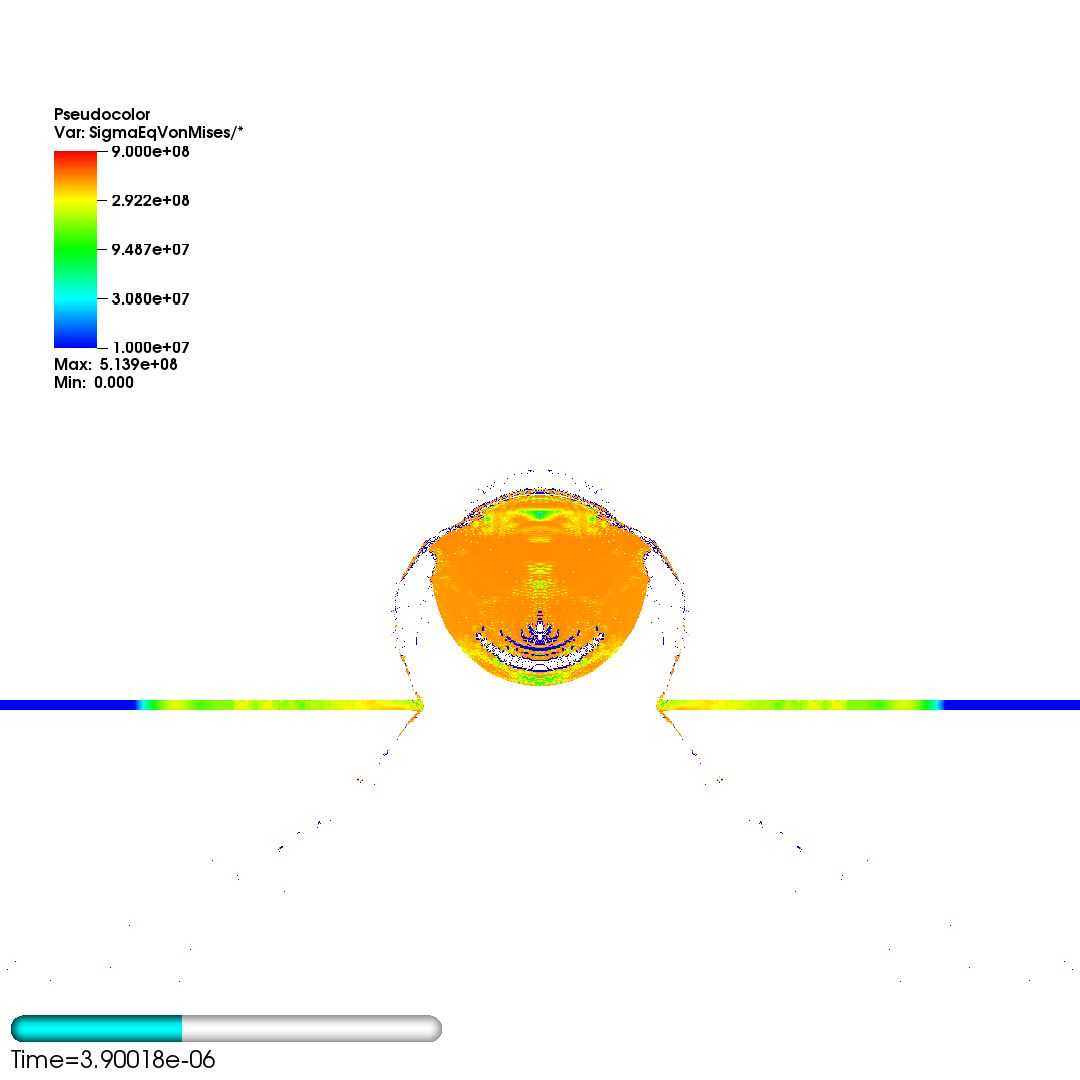
ABSTRACT: A simulation of a simple penetration experiment is performed using Material Point Method (MPM) through the Uintah Computational Framework (UCF) and interpreted using the post-processing visualization program VisIt. MPM formatting sets a background mesh with explicit boundaries and monitors the interaction of particles within that mesh to predict the varying movements and orientations of a material in response to loads. The modeled experiment compares the effects of an aluminum sphere impacting an aluminum sheet at varying velocities. In this work, the experiment called launch T-1428 (by Piekutowski and Poorman) is simulated using UCF and VisIt. The two materials in the experiment are both simulated using a hypoelastic-plastic model. Varying grid resolutions were used to verify the convergent behavior of the simulations to the experimental results. The validity of the simulation is quantified by comparing perforation hole diameter. A full 3-D simulation followed and was also compared to experimental results. Results and issues in both 2-D and 3-D simulation efforts are discussed. Both the axisymmetric and 3-D simulation results provided very good data with clear convergent behavior.
See the link below for the full report.
NEWS FLASH: The print version of the Meyer-Brannon paper on statistical variation of fracture patterns in a continuum code (CTH) is now available at http://dx.doi.org/10.1016/j.ijimpeng.2010.09.007.

Perforation with Aleatory Uncertainty of high-pressure strength in an Eulerian Simulation.

Stress net view of maximum shear lines inferred from molecular dynamics simulation of crack growth. Image from http://doi.ieeecomputersociety.org/10.1109/VIS.2005.33

Brazilian stress net before and after material failure. Colors indicate maximum principal stress (showing tension in the center of this axially compressed disk). Lines show directions of max principal stress.
A stress net is simply a graphical depiction of principal stress directions (or other directions derived from them, such as rotating them by 45 degrees to get the maximum shear lines.) Continue reading

Stills from YouTube video of buried roadside explosive
As one of four institutions collaborating with the University of Colorado — Boulder, the CSM group in the Department of Mechanical Engineering at the University of Utah, will be developing constitutive models for soils, as well as full-scale simulation capabilities in Uintah to predict blast and ejecta from shallow buried explosives (such as roadside improvised explosive devices). The $1.1M slated for CSM work presumes the project will last 5 years. For more information, see the University of Colorado’s press release.

The straight line is the linear regression of a function that takes scalars (x-values) as input and returns scalars (y-values) as output. (figure from GANFYD)
You’ve probably seen classical equations for linear regression, which is a procedure that finds the straight line that best fits a set of discrete points 


The pink parallelogram is the multi-linear regression of a function that takes vectors (gray dots) as input and returns vectors (blue dots) as output
The bottom of this post provides a link to a tutorial on how to generalize the concept of linear regression to fit a function 


Constitutive modeling refers to the development of equations describing the way that materials respond to various stimuli. In classical deformable body mechanics, a simple constitutive model might predict the stress required to induce a given strain; the canonical example is Hooke’s law of isotropic linear elasticity. More broadly, a constitutive model predicts increments in some macroscale state variables of interest (such as stress, entropy, polarization, etc.) that arise from changes in other macroscale state variables (strain, temperature, electric field, etc.).
Constitutive equations are ultimately implemented into a finite element code to close the set of equations required to solve problems of practical interest. This course describes a few common constitutive equations, explaining what features you would see in experimental data or structural behavior that would prompt you to select one constitutive model over another, how to use them in a code, how to test your understanding of the model, how to check if the code is applying the model as advertised in its user’s manual, and how to quantitatively assess the mathematical and physical believability of the solution.
M.Y. Lee, R.M. Brannon and D.R. Bronowski

Explosive failure of the SICN-UC02 specimen (12.7 mm in diameter and 25.4 mm in length) subjected to the unconfined uniaxial compressive stress condition
To establish mechanical properties and failure criteria of silicon carbide (SiC-N) ceramics, a series of quasi-static compression tests has been completed using a high-pressure vessel and a unique sample alignment jig. This report summarizes the test methods, set-up, relevant observations, and results from the constitutive experimental efforts. Combining these quasistatic triaxial compression strength measurements with existing data at higher pressures naturally results in different values for the least-squares fit to this function, appropriate over a broader pressure range. These triaxial compression tests are significant because they constitute the first successful measurements of SiC-N compressive strength under quasistatic conditions. Having an unconfined compressive strength of ~3800 MPa, SiC-N has been heretofore tested only under dynamic conditions to achieve a sufficiently large load to induce failure. Obtaining reliable quasi-static strength measurements has required design of a special alignment jig and loadspreader assembly, as well as redundant gages to ensure alignment. When considered in combination with existing dynamic strength measurements, these data significantly advance the characterization of pressure-dependence of strength, which is important for penetration simulations where failed regions are often at lower pressures than intact regions.
Available Online:
http://www.mech.utah.edu/~brannon/pubs/2004LeeBrannonBronowskiTriaxTestsSiC.pdf
http://www.osti.gov/bridge/purl.cover.jsp?purl=/920770-6YyIPp/
H.W. Meyer Jr. and R.M. Brannon
[This post refers to the original on-line version of the publication. The final (paper) version with page numbers and volume is found at http://dx.doi.org/10.1016/j.ijimpeng.2010.09.007. Some further details and clarifications are in the 2012 posting about this article]

Simulation results for a reference volume of 0.000512 cm^3 ; sf is the size effect factor
Continuum mechanics codes modeling failure of materials historically have considered those materials to be homogeneous, with all elements of a material in the computation having the same failure properties. This is, of course, unrealistic but expedient. But as computer hardware and software has evolved, the time has come to investigate a higher level of complexity in the modeling of failure. The Johnsone-Cook fracture model is widely used in such codes, so it was chosen as the basis for the current work. The CTH finite difference code is widely used to model ballistic impact and penetration, so it also was chosen for the current work. The model proposed here does not consider individual flaws in a material, but rather varies a material’s Johnsone-Cook parameters from element to element to achieve in homogeneity. A Weibull distribution of these parameters is imposed, in such a way as to include a size effect factor in the distribution function. The well-known size effect on the failure of materials must be physically represented in any statistical failure model not only for the representations of bodies in the simulation (e.g., an armor plate), but also for the computational elements, to mitigate element resolution sensitivity of the computations.The statistical failure model was tested in simulations of a Behind Armor Debris (BAD) experiment, and found to do a much better job at predicting the size distribution of fragments than the conventional (homogeneous) failure model. The approach used here to include a size effect in the model proved to be insufficient, and including correlated statistics and/or flaw interactions may improve the model.
Available Online:
http://www.mech.utah.edu/~brannon/pubs/7-2011MeyerBrannon_IE_1915_final_onlinePublishedVersion.pdf
http://www.sciencedirect.com/science/article/pii/S0734743X10001466
A. Sadeghirad, R. M. Brannon, and J. Burghardt

Three snapshots of the model with 248 particles in simulation of the radial expansion of a ring problem using: (a) CPDI method and (b) cpGIMP
A new algorithm is developed to improve the accuracy and efficiency of the material point method for problems involving extremely large tensile deformations and rotations. In the proposed procedure, particle domains are convected with the material motion more accurately than in the generalized interpolation material point method. This feature is crucial to eliminate instability in extension, which is a common shortcoming of most particle methods. Also, a novel alternative set of grid basis functions is proposed for efficiently calculating nodal force and consistent mass integrals on the grid. Specifically, by taking advantage of initially parallelogram-shaped particle domains, and treating the deformation gradient as constant over the particle domain, the convected particle domain is a reshaped parallelogram in the deformed configuration. Accordingly, an alternative grid basis function over the particle domain is constructed by a standard 4-node finite element interpolation on the parallelogram. Effectiveness of the proposed modifications is demonstrated using several large deformation solid mechanics problems.
Available Online:
http://www.mech.utah.edu/~brannon/pubs/7-2011-SadeghiradBrannonBurghardt-NME.pdf
http://onlinelibrary.wiley.com/doi/10.1002/nme.3110/abstract

