Transform between a cube’s surface and a square

I plan to add this transformation to my upcoming book on computational geometry. This mapping was originally conceived to provide a one-to-one correspondence between RGB color and locations on a dance floor for a positioning correction in a project on robotic square dancers, but then we realized that simply laying down QR codes with coordinate and orientation data would be far more accurate.
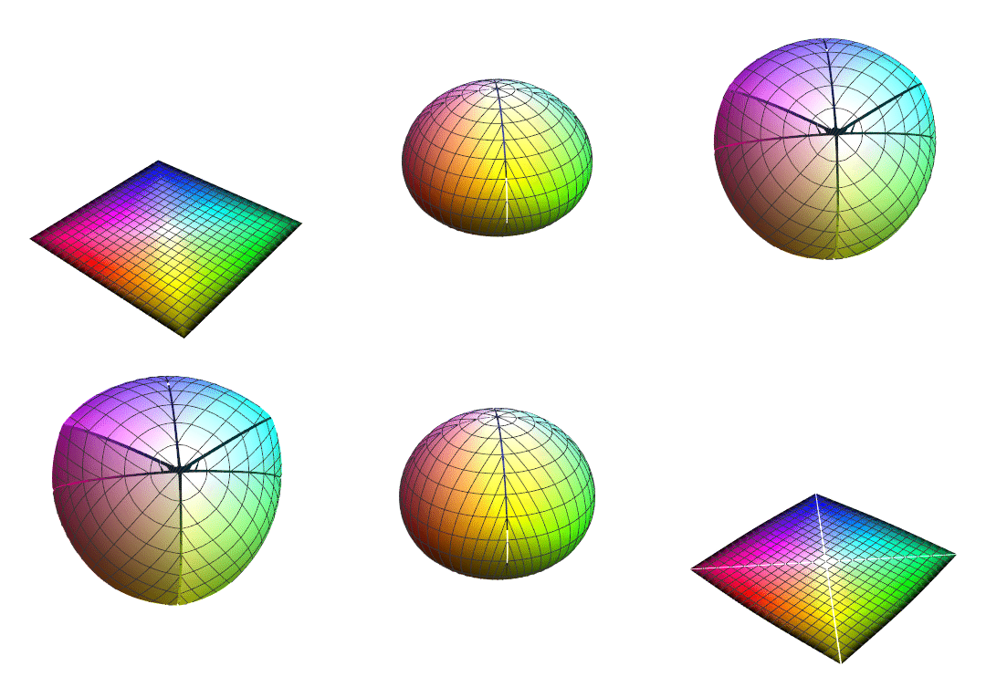
So what might be a good application for this transformation? It essentially maps the surface of the RGB cube (i.e., all fully saturated colors) to a square. One possibility would be to extend color plots that are conventionally used to depict one one variable to instead show two variables. In mechanics, for example, engineers typically show two different color plots for pressure and temperature, each with its own a linear legend bar ranging from a logical coordinate eta from 0 to 1, which is mapped to a selected linear color scheme (such as “hue” to range over the rainbow). In the single-variable color plots, the value of eta is set in proportion to the variable being plotted. To avoid needing two separate color plots for pressure and temperature a square color legend could be used with coordinates (eta1, eta2) associated with the two variables. While a “poor man’s” color plot mapping could be RGB[0,eta1,eta2], the one shown here would be far more spectacular because it would represent the full range of fully saturated colors (without “muddy” colors in the interior of the RGB cube) and, furthermore, values outside the range of interest would show as black.

CPDI shape functions for the Material Point Method

In a conventional MPM formulation, the shape functions on the grid are the same as in a traditional FEM solution. In the CPDI, the shape functions on the grid are replaced by alternative (and still linearly complete*) shape functions, given by piecewise linear interpolations of the traditional FEM shape functions to the boundaries of the particles.  This change provides FEM-level accuracy in moderately deforming regions while retaining the attractive feature of MPM that particles can move arbitrarily relative to one another in massively deforming regions (provided, of course, that the deformation is updated in a manner compatible with the constitutive model).

In the images below, the shaded regions are the traditional FEM “tent” linear shape functions in 1-D, and the solid lines are the CPDI interpolated shape functions, which clearly change based on particle position relative to the grid.  Both the traditional FEM tent functions and these new CPDI functions are linearly complete (i.e., they can exactly fit any affine function). The tremendous advantage of CPDI is that the basis functions are extraordinarily simple over a particle domain, thus facilitating exact and efficient evaluation of integrals over particle domains.

Continue reading

Research: Radial cracking as a means to infer aleatory uncertainty parameters

Aleatory uncertainty in constitutive modeling refers to the intrinsic variability in material properties caused by differences in micromorphology (e.g., grain orientation or size, microcracks, inclusions, etc.) from sample to sample. Accordingly, a numerical simulation of a nominally axisymmetric problem must be run in full 3D (non-axisymmetric) mode if there is any possibility of a bifurcation from stability.

Dynamic indentation experiments, in which a spherical ball impacts to top free surface of a cylindrical specimen, nicely illustrate that fracture properties must have spatial variability — in fact, the intrinsic instability that leads to radial cracking is regarded by the Utah CSM group as a potential inexpensive means of inferring the spatial frequency of natural variations in material properties.

Radial cracking in dynamic indentation experiments.

Continue reading

Verification Research: The method of manufactured solutions (MMS)


MMS stands for “Method of Manufactured Solutions,” which is a rather sleazy sounding name for what is actually a respected and rigorous method of verifying that a finite element (or other) code is correctly solving the governing equations.

A simple introduction to MMS may be found on page 11 of The ASME guide for verification and validation in solid mechanics. The basic idea is to analytically determine forcing functions that would lead to a specific, presumably nontrivial, solution (of your choice) for the dependent variable of a differential equation.  Then you would verify a numerical solver for that differential equation by running it using your analytically determined forcing function.  The difference between the code’s prediction and your selected manufactured solution provides a quantitative measure of error.

Continue reading

Stress State Analysis Python Script

General Mohr's Circle for 3D Stress State

General Mohr's Circle for 3D Stress State

Have you ever had a stress state and wanted to simply get the principal stresses without finding a web applet to do it for you? Or maybe you want to know what the deviatoric part of the stress is without finding and using a copy of MATLAB or Mathematica to do the matrix operations for you? This script was written to help answer those questions in as little time as possible with an intuitive command line input syntax.

This script was written in Python (www.python.org) and makes use of the NumPy module (www.numpy.scipy.org). Python is a fairly platform independent programming language with more and more programs being dependent on it on all platforms. The NumPy module adds significant scientific computation power to the language by adding N-dimensional matrix support, matrix operations, LAPACK functions (matrix inverse, eigenvalue and eigenvector decompositions, etc.), among other things.

You can download the script here.

Continue reading

Tutorial: Emacs and GDB

I remember learning how to use a debugger and Utah State University as an undergraduate.  We learned to program in Fortran 90, and used a Microsoft debugger.  It seemed cool, but honestly with the types of programs I was writing at the time, using print statement seemed to be effective enough and less of a hassle.  Recently I have been working with the Uintah MPM code, which is MUCH larger and more complex than any code I’ve ever written.  After several months of wading through the code I finally came across a problem that “cout” just could not help me solve.  The code was suddenly crashing with an allocation error and giving no useful backtrace information.  A colleague suggested that I use gdb to find out where the problem was occurring.  It turned out to be very, very helpful and surprisingly easy to use.  I’ve recently become a convert to Emacs, and found that the gdb interface in Emacs is especially nice.  So here is goes:

Continue reading