MMS stands for “Method of Manufactured Solutions,” which is a rather sleazy sounding name for what is actually a respected and rigorous method of verifying that a finite element (or other) code is correctly solving the governing equations.

A simple introduction to MMS may be found on page 11 of The ASME guide for verification and validation in solid mechanics. The basic idea is to analytically determine forcing functions that would lead to a specific, presumably nontrivial, solution (of your choice) for the dependent variable of a differential equation.  Then you would verify a numerical solver for that differential equation by running it using your analytically determined forcing function.  The difference between the code’s prediction and your selected manufactured solution provides a quantitative measure of error.

In SOLID MECHANICS, the primary governing equation is the balance of linear momentum,

The remaining governing equations are conservation of mass and the constitutive model (e.g., Hooke’s Law of elasticity).

Codes that solve these equations are typically written under the assumption that applied loads (surface tractions and body forces) are known, possibly along with some known displacements or velocities, typically at the boundary.  The solution sought by these codes is the time varying displacement of all points in the domain.

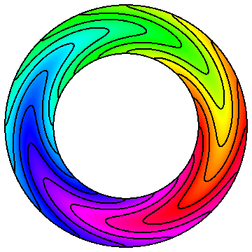
The method of manufactured solutions (MMS) reverses this scenario. In the MMS, a time-varying displacement field is constructed (i.e., a solution is “manufactured”) based on the whims of the analyst. It might be like the one illustrated in the animation shown above.  With the manufactured solution pre-determined and presumably well behaved enough for you to perform calculus on it, you can differentiate it twice with respect to time to determine the acceleration. Likewise, you can take its gradient to determine the strain field (or any other displacement-dependent fields) from which you can apply the constitutive model to get stress. By taking the divergence of the analytically determined stress field that goes with your manufactured solution, you can ultimately use the momentum equation to solve for the body force field.

In the MMS code-verification phase, you use the analytically determined body force field, as well as boundary tractions, as the forcing functions in your code.  You may then declare that the code is running correctly (at least for this problem) if its prediction for the displacement field is the original manufactured displacement field that you dreamed up. Otherwise, the code is either solving the equations inaccurately or you made some mistake in your analytical determination of the body force, or you made a user error implementing the body force itself (or other input) in the code. Since the exact solution is known, this MMS technique allows you to make quantiative assessments of accuracy for nontrivial problems.

ADVANTAGES OF THE “VORTEX RING” MANUFACTURED SOLUTION
The illustrated vortex ring problem moves material points around in circles so that every material point is in a state of differing intensities of simple shear with differing amounts of superimposed rotation. The color in the animation is just the initial angle (to better visualize this motion); the black lines show the differing amounts of circumferential movement. A working implementation of the illustrated vortex ring verification test (along with a copy of the publication), is found in our free matlab MPM code. Above, the domain is a ring, but it can be easily extended to a full rectangular domain.

In dynamics codes, especially if they are not finite element codes (e.g., if they are particle codes or Eulerian hydrocodes), traction and displacement boundary conditions can be very difficult to enforce; in fact many of these codes provide support for only one type of boundary condition: traction-free. For this reason, the generalized vortex ring illustrated at the top of this post can be very useful. If you look carefully at that deformation, you will notice that both displacement and strain are zero at the boundaries of the ring, hence corresponding to zero traction boundary conditions, which are often called “natural” boundary conditions since they require no special handling in most numerical momentum solvers.  As a matter of fact, the vortex ring domain may be extended to become a simple square domain as illustrated below. If you use your code to run the problem shown below (i.e., the vortex ring on a square domain), you will probably see motion of material away from the ring, which is a nice visual depiction of solution error (since the manufactured exact solution has no motion there).

Another attraction of the problem illustrated in this post is that all points are undergoing essentially the same class of deformation: simple shear with superimposed rotation. Thus, this problem not only helps to investigate if your code can handle massively large deformations similar to what is typical in penetration simulations, it also confirms that your code has basis invariance (i.e., not getting different results at different polar angles) and frame indifference (i.e., transforming the predicted stresses properly under superimposed rotation of the sheared state as it moves around the ring).

Follow-up posts describe this problem in greater detail, showing the results of using it to test both finite-element codes and research particle method codes.