Have you ever had a stress state and wanted to simply get the principal stresses without finding a web applet to do it for you? Or maybe you want to know what the deviatoric part of the stress is without finding and using a copy of MATLAB or Mathematica to do the matrix operations for you? This script was written to help answer those questions in as little time as possible with an intuitive command line input syntax.

This script was written in Python (www.python.org) and makes use of the NumPy module (www.numpy.scipy.org). Python is a fairly platform independent programming language with more and more programs being dependent on it on all platforms. The NumPy module adds significant scientific computation power to the language by adding N-dimensional matrix support, matrix operations, LAPACK functions (matrix inverse, eigenvalue and eigenvector decompositions, etc.), among other things.

You can download the script here.

Script Usage

Let’s analyze the following symmetric stress matrix:

With this command (in linux):

> ./stress.py sig11 sig22 sig33 sig12 sig13 sig23

Or, if there are no off-diagonal components:

> ./stress.py sig11 sig22 sig33

Let’s assume that , , and all remaining entries are equal to zero (with units of stress in whatever system you prefer). We do this with the following command (again in linux):

> ./stress.py 1 0 3 0 2 0

and would get the output that is found at the bottom of this post.

How are these values computed?

Isotropic and Deviatoric Parts of the Stress State

For our stress matrix , we can find the isotropic part by the following matrix formula:

Where is the trace operator and is the 3×3 identity matrix.
The isotropic and deviatoric parts of stress add to the original stress matrix. So, we can find the deviatoric part of the stress state by:

Stress Invariants: , , and

We will simply define the invariants here, primarily for computing other, more physically meaningful values.

The Principal Stresses: P1, P2, and P3

The principal stresses are computed from performing an eigenvalue decomposition on the stress matrix and then sorting those values. This eigendecomposition is done by using a built-in function that is a part of the NumPy module. We’ll call these ordered principal stresses , , and for the rest of this discussion. Because they are ordered, the stresses are . These values can be found in the general image of Mohr’s circle below as the intersection points of the three circles with the axis.

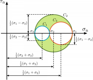
Maximum Shear

This is found by:

It can also be found graphically as the radius of the largest circle in the image of Mohr’s circle below.

Mean Stress

This is found by finding the average stress, using either the average of the principal stresses or one third of the trace (both are equivalent):

This can also be found graphically as the center of the largest circle in the image of Mohr’s circle, below.

For additional information on Mohr’s Circle, there is a wonderful full PDF writeup available here.

Equivalent Stress

The long way to find the equivalent stress is:

But can also be found using a stress invariant:

Lode Coordinates

Lode coordinates are a useful basis for describing states of stress. We take the three principal stresses and then cast them in terms of , , and . However, instead of taking to be in the direction of one of the principal stresses, it points along the principal space diagonal (along the in principal stress space).

Triaxiality

Triaxiality is the ratio of mean stress to equivalent stress or, in other words, the ratio of the lode coordinates to and is usually designated by the greek letter . Specifically:

Example Script Output

From the above example, if we run

> ./stress.py 1 0 3 0 2 0

We get this as output:

===================== Stress State Analysis ====================

Input Stress:
[[ 1.  0.  2.]
 [ 0.  0.  0.]
 [ 2.  0.  3.]]

====================== Component Matricies =====================

Isotropic Stress:
[[ 1.33333333  0.          0.        ]
 [ 0.          1.33333333  0.        ]
 [ 0.          0.          1.33333333]]
Deviatoric Stress:
[[-0.33333333  0.          2.        ]
 [ 0.         -1.33333333  0.        ]
 [ 2.          0.          1.66666667]]

========================= Scalar Values ========================

                            P1:  4.2360679775e+00
                            P2:  0.0000000000e+00
                            P3: -2.3606797750e-01
                     Max Shear:  2.2360679775e+00
                   Mean Stress:  1.3333333333e+00
             Equivalent Stress:  4.3588989435e+00
                            I1:  4.0000000000e+00
                            J2:  6.3333333333e+00
                            J3:  6.0740740741e+00
                        Lode z:  2.3094010768e+00
                        Lode r:  3.5590260840e+00
              Lode theta (rad):  4.7667961159e-01
              Lode theta (deg):  2.7311729924e+01
                   Triaxiality:  3.0588764516e-01

========================== End Output ==========================