Publication: Verification tests in solid mechanics

ABSTRACT: Code verification against analytical solutions is a prerequisite to code validation against experimental data. Though solid-mechanics codes have established basic verification standards such as patch tests and convergence tests, few (if any) similar standards exist for testing solid-mechanics constitutive models under nontrivial massive deformations. Increasingly complicated verification tests for solid mechanics are presented, starting with simple patch tests of frame-indifference and traction boundary conditions under affine deformations, followed by two large-deformation problems that might serve as standardized verification tests suitable to quantify accuracy, robustness, and convergence of momentum solvers used in solid-mechanics codes. These problems use an accepted standard of verification testing, the method of manufactured solutions (MMS), which is rarely applied in solid mechanics. Body forces inducing a specified deformation are found analytically by treating the constitutive model abstractly, with a specific model introduced only at the last step in examples. One nonaffine MMS problem subjects the momentum solver and constitutive model to large shears comparable to those in penetration, while ensuring natural boundary conditions to accommodate codes lacking support for applied tractions. Two additional MMS problems, one affine and one nonaffine, include nontrivial traction boundary conditions.

For a copy of the paper along an implementation of the vortex problem, see our simple matlab MPM code.

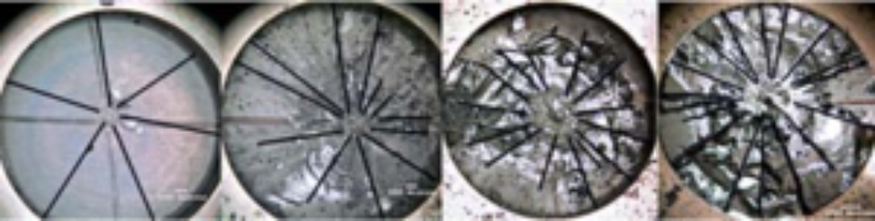
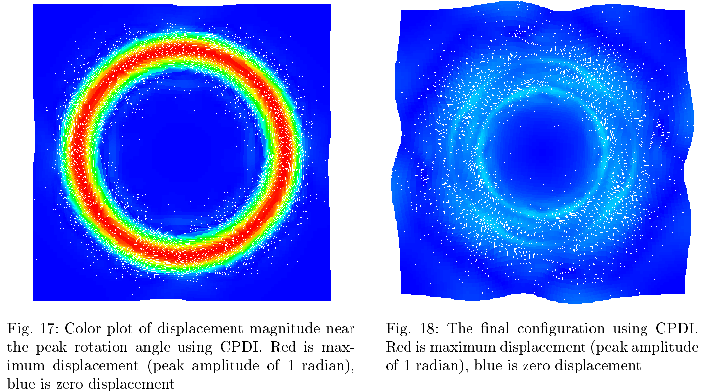
Here are some eye-catching graphics (see the paper itself for details):

2013verificationPic1 Continue reading

Publication: Aleatory quantile surfaces in damage mechanics

ABSTRACT: In statistical damage mechanics, a deterministic failure limit surface is replaced with a scale-dependent family of quantile surfaces. An idealized homogeneous isotropic matrix material containing cracks of random size and orientation is used to elucidate expected mathematical character
of aleatory uncertainty and scale effects for initiation of damage in a brittle material. Scope is limited to statistics and scale dependence for the ONSET (not subsequent progression) of shear-driven failure. Exact analytical solutions for probability of such failure (with an interesting pole-point visualization) are derived for axisymmetric extension or compression of a single-crack sample. A semi-analytical bound on the failure CDF is found for a multi-crack specimen by integrating the single-crack probability over an exponential crack size distribution for which the majority of flaws are small enough to be safe from failure at any orientation. Resulting tails of the predicted failure distribution differ from Weibull theory,
especially in the third invariant.

Selected cool pictures (see the article for more images):

2014AleatoryQuantileSurfacesPic1

Continue reading

Public display of affection for Prof. Gib Richards

Dear Prof. Richards:

When I was still a teenager, you were my undergraduate advisor at the University of New Mexico (UNM). While seated in your office surrounded by rubber chickens, whoopee cushions, and other fanciful toys (which you had because of your side hobby of being a clown), I asked: “How can I know if I will ultimately enjoy a career in Mechanical Engineering?” You replied: “If you are willing to graduate one or two semesters late, then you can find the answer to that question by doing a co-op student internship.” To prepare me for this opportunity, your first action was to help me get a local internship at the Air Force Research Laboratory (then named Weapons Laboratory) at Kirtland AFB. You made telephone calls and otherwise worked your magic to get me into a co-op during the next summer at Los Alamos National Laboratory, where I quickly came to realize that it was the PhDs who were doing the most interesting and self-directed work. I also learned at Los Alamos that educated people have the self-discipline to NOT SMOKE CIGARETTES and to NOT USE SWEAR WORDS. My supervisor at Los Alamos furthermore advised me to go back to UNM and take as many classes as possible from Buck Schreyer, which likewise delightfully shaped my career. Thus, Prof. Richards, you deserve more credit than anyone else for pointing me in the direction of a healthy PhD track, ultimately leading to 14 years as a researcher at Sandia National Laboratories and (most recently) as a professor of Mechanical Engineering since 2007.

I still fondly recall being the first of your students to use computer-generated graphics and laser printing in my senior research report, but that didn’t distract you from fulfilling your promise to find ten grammar/spelling errors. Did you ever fail in that quest with any other student? You were the person who graded my co-op report upon my return to UNM, where you taught me that “finite elements” is only *sometimes* hyphenated, consequently launching a campaign of my own to explain hyphenation rules to others (see, for example, my blog article https://csmbrannon.net/2013/08/04/hyphenation-in-technical-or-other-writing/).

In summary, Prof. Richards, you have profoundly influenced my life! I love you for everything you have done for me and for countless other students.

Sincerely, Rebecca Brannon

Holey Particle Basis functions for 2D CPDI

allpictab

An older post (https://csmbrannon.net/2013/09/29/particle-basis-function-in-the-cpdi-method/) showed particle basis functions in 1D, demonstrating that they retain overlapping support with neighboring particles when using CPDI even when the particles are stretched to be large multiples of the grid cell length. In the 1D context of those examples, “holes” in CPDI basis functions are impossible.

This post shows an extreme 2D example (suggested by John Nairn, Jim Guilkey, and Michael Homel*) that can deleteriously lose overlapping support of particle shape functions, which can then allow non-physical material interpenetration.

Continue reading

PowerPoint slides for Mohr’s circle

The link below provides a collection of slides used to explain Mohr’s circle in an undergraduate mechanics course at the University of Utah.  If you use a Mac, it is unlikely that these will render properly (so go sit at a PC in your university computer lab to look at them).  Make sure to use slideshow mode, as these have many animations!

MohrCircleFiles  (zip file contains two PPT lectures and one Mathematica file)

F-tables for prescribed deformation

Motion without superimposed rotation

Motion without superimposed rotation

Same deformation with superimposed rotation

Same deformation with superimposed rotation

When developing constitutive models, it is crucial to run the model under a variety of standard (and some nonstandard) homogeneous deformations. To do this, you must first describe the motion mathematically. As indicated in http://csm.mech.utah.edu/content/wp-content/uploads/2011/03/GoBagDeformation.pdf, a good way to do that is to give the deformation gradient tensor, F. The component matrix [F] contains the deformed edge vectors of an initially unit cube, making this a very easy to way to prescribe deformations.

Continue reading

Particle basis function in the CPDI method

The Convected Particle Domain Interpolation (CPDI) method for evaluating nodal integrals in the weak form of the momentum equation employs a dynamically adaptive alternative to standard shape functions on the grid. The CPDI basis functions change depending on the underlying particle morphology.  The animations in this post each provide image triplet groupings, one triplet for pure translation and the other for uniform stretching, defined as follows:

  • TOP IMAGE: The dynamic CPDI basis (solid lines) compared with the conventional FEM-style basis functions (shaded tent functions). The adaptive CPDI basis is constructed to exactly coincide with the conventional FEM basis at particle edges (called corners), and it varies linearly across each particle domain, thus making integrals of the basis or its gradient over a particle domain quite simple. The CPDI basis is linearly complete.
  • MIDDLE IMAGE: The particle basis (shown shaded in dark gray). Like the CPDI basis itself, the particle basis is never constructed explicitly. We are visualizing it here to better understand the domain of influence of a particle and (we hope) to discourage the mysterious tendency for researchers to refer to \phi_i(x_p)=\frac{1}{V_p}\int_{\Omega_p(x_p)}S_i(x)dx as the particle basis function.  To the contrary, and as explained in detail in the bottom of this post, the particle basis function is the coefficient of the particle data value appearing in an expansion of a field as it is used in the discretization of governing equations.  The solution of the governing equations uses a mapping of particle data to the grid. Consequently, because all fields are treated as expansions on the grid, the particle basis function (found by setting the particle value to 1 and all other particle data to zero) must be a grid expansion (so it MUST be piecewise linear on the grid if using linear shape functions).  This proper definition of the particle basis function is shown below in dark gray. The particle basis function is NOT the top hat function (shown in light gray), nor is it \phi_{ip} as commonly and misleadingly asserted. The relatively complicated derivation of the particle basis function is provided at the bottom of this post.  In the images below, two options are considered for the mapping u_p particle data to the grid nodal value u_i=\sum_p\psi_{pi}^*u_p:
    • Option 1: \psi_{pi}^*=\frac{\phi_{ip}^*}{\sum_p\phi_{ip}}
    • Option 2: \psi_{pi}^* is taken as the pseudo-inverse of \phi_{ip}^*

Here, \phi_{ip}^* is the average of the ith CPDI grid nodal basis function, S_i^*(x) 
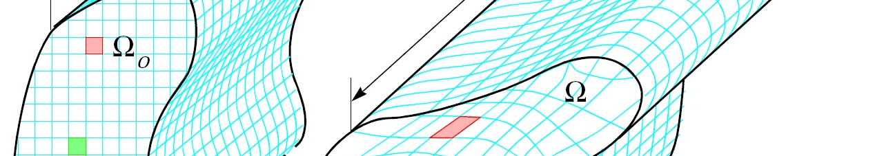
over the pth particle domain \Omega_p. The GIMP variants of MPM  are similar except that they evaluate \phi_{ip} and \psi_{pi} using the conventional S_i(x) grid basis functions rather than the adaptive (and actually computationally simpler) ones used in CPDI. Legacy “standard” MPM evaluates \phi_{ip} to merely equal S_i(x_p), which causes grid-crossing errors. The figure groupings below use the CPDI formula
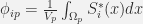
 \phi_{ip}=\frac{1}{V_p}\int_{\Omega_p}S_i^*(x) dx in which S_i^*(x) is the CPDI adaptive grid basis. The MIDDLE image in each image triplet shows the particle basis, which is constructed by applying the above mapping to the grid with all particle values set to 0 except 1 at the particle of interest. The light grey filled box in the middle image shows a piecewise constant description (=1 on the particle domain and 0 elsewhere), while the dark filled function is the associated particle basis on the grid. The dots show nodal values of the particle basis function to emphasize that nodal values are not equal to field values (there is no need for them to be). Seeing a nodal value “pop up” gives you a sense of when a particle begins to influence the field in grid cells containing that node. The other (colored) graphs in that plot are the similarly constructed basis functions for the other particles. As seen in the upcoming plots, OPTION 2 (the pseudo-inverse) produces particle basis functions that are neither positive everywhere nor of compact support (which could be problematic for parallelisation in applications).

  • The BOTTOM row in each grouping of plots shows the representations of a field that is constant (at particles) and a field that linearly varying from 0 to 1 over the physical domain (with particle values set equal to that field at the particle location). As seen, OPTION 2 for setting \psi_{pi}^* gives excellent results for the linear field when there are at least two particles per cell, but OPTION 1 seems to be a better overall choice because it gives good results for any particle density, including fractional particles per cell (desired for coarse descriptions in regions of little interest). Grid errors at boundaries with OPTION 1 could probably be reduced by enriching boundary particles (as described in the CPDI2 publication), but this remains to be proved.

Continue reading