Tutorial: Visualizing Deformation

If you’ve never heard of a continuum mapping, read our introduction to mappings.

This posting discusses the two most common visualization methods for 3D homogeneous mappings: Showing how a sphere transforms to an ellipsoid and how a cube transforms to a parallelepiped:
Sphere transforming to ellipsoidBox transforming to parallelepiped

Continue reading

Resource: Perfect triples, “nice” unit vectors, and “nice” orthogonal matrices

“NICE” lists:

Perfect Triangles

Perfect Triangles

Have you ever noticed that textbooks often involve so-called 3-4-5 triangles? They do that to make the algebraic manipulations easier for students.  If the two legs of a right triangle are of length 3 and 4, then the hypotenuse (found from the Pythagorean theorem) has a length of 5, which is “nice” in the sense that it is an integer rather than an irrational square root that more typically comes from solving the Pythagorean theorem. As discussed in many elementary math sites (such as MakingMathematics.org), another example of a “nice” triangle is the 5-12-13 triangle, since 5^2+12^2=13^2 .

The external links in this posting contain a list of more of these so-called perfect triples of integers \{a,b,c\} for which a^2+b^2=c^2 . Perfect triples are also used to create “nice” 2D unit vectors whose components are each rational numbers (instead of involving irrational square roots from the normalization process). For example, the classic unit vector based on the 3-4-5 perfect triple is simply \{\frac{3}{5},\frac{4}{5}\} . Continue reading

Tutorial: multi-linear regression

The straight line is the linear regression of a function that takes scalars (x-values) as input and returns scalars (y-values) as output. (figure from GANFYD)

You’ve probably seen classical equations for linear regression, which is a procedure that finds the straight line that best fits a set of discrete points \{(x_1,y_1), (x_2,y_2),...,(x_N,y_N)\} . You might also be aware that similar formulas exist to find a straight line that is a best (least squares) fit to a continuous function y(x) .

The pink parallelogram is the multi-linear regression of a function that takes vectors (gray dots) as input and returns vectors (blue dots) as output

The bottom of this post provides a link to a tutorial on how to generalize the concept of linear regression to fit a function \vec{y}(\vec{x}) that takes a vector \vec{x} as input and produces a vector \vec{y} as output. In mechanics, the most common example of this type of function is a mapping function that describes material deformation: the input vector is the initial location of a point on a body, and the output vector is the deformed location of the same point. The image shows a collection of input vectors (initial positions, as grey dots) and a collection of output vectors (deformed locations as blue dots). The affine fit to these descrete data is the pink parallelogram. Continue reading

Course offering: ME 7960 (special topics) Computational Constitutive Modeling

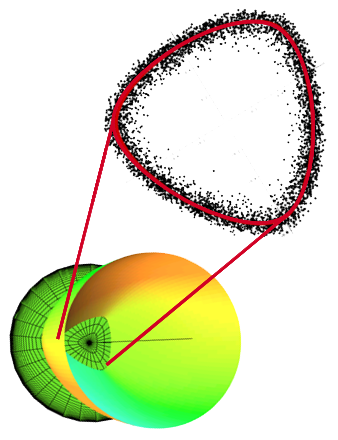
Third invariant yield surface with uncertainty

Constitutive modeling refers to the development of equations describing the way that materials respond to various stimuli. In classical deformable body mechanics, a simple constitutive model might predict the stress required to induce a given strain; the canonical example is Hooke’s law of isotropic linear elasticity. More broadly, a constitutive model predicts increments in some macroscale state variables of interest (such as stress, entropy, polarization, etc.) that arise from changes in other macroscale state variables (strain, temperature, electric field, etc.).

Constitutive equations are ultimately implemented into a finite element code to close the set of equations required to solve problems of practical interest. This course describes a few common constitutive equations, explaining what features you would see in experimental data or structural behavior that would prompt you to select one constitutive model over another, how to use them in a code, how to test your understanding of the model, how to check if the code is applying the model as advertised in its user’s manual, and how to quantitatively assess the mathematical and physical believability of the solution.

Continue reading

Publication: Uniaxial and Triaxial Compression Tests of Silicon Carbide Ceramics under Quasi-static Loading Condition

M.Y. Lee, R.M. Brannon and D.R. Bronowski

Explosive failure of the SICN-UC02 specimen (12.7 mm in diameter and 25.4 mm in length) subjected to the unconfined uniaxial compressive stress condition

To establish mechanical properties and failure criteria of silicon carbide (SiC-N) ceramics, a series of quasi-static compression tests has been completed using a high-pressure vessel and a unique sample alignment jig.  This report summarizes the test methods, set-up, relevant observations, and results from the constitutive experimental efforts. Combining these quasistatic triaxial compression strength measurements with existing data at higher pressures naturally results in different values for the least-squares fit to this function, appropriate over a broader pressure range. These triaxial compression tests are significant because they constitute the first successful measurements of SiC-N compressive strength under quasistatic conditions. Having an unconfined compressive strength of ~3800 MPa, SiC-N has been heretofore tested only under dynamic conditions to achieve a sufficiently large load to induce failure. Obtaining reliable quasi-static strength measurements has required design of a special alignment jig and loadspreader assembly, as well as redundant gages to ensure alignment. When considered in combination with existing dynamic strength measurements, these data significantly advance the characterization of pressure-dependence of strength, which is important for penetration simulations where failed regions are often at lower pressures than intact regions.

Available Online:

http://www.mech.utah.edu/~brannon/pubs/2004LeeBrannonBronowskiTriaxTestsSiC.pdf

http://www.osti.gov/bridge/purl.cover.jsp?purl=/920770-6YyIPp/

Publication: Experimental Assessment of Unvalidated Assumptions in Classical Plasticity Theory

R. Brannon, J.A. Burghardt, D. Bronowski, and S. Bauer

Common isotropic yield surfaces. Von Mises and Drucker-Prager models are often used for metals. Gurson’s function, and others like it, are used for porous media. Tresca and Mohr-Coulomb models approximate the yield threshold for brittle media. Fossum’s model, and others like it, combine these features to model realistic geological media.

This report investigates the validity of several key assumptions in classical plasticity theory regarding material response to changes in the loading direction. Three metals, two rock types, and one ceramic were subjected to non-standard loading directions, and the resulting strain response increments were displayed in Gudehus diagrams to illustrate the approximation error of classical plasticity theories. A rigorous mathematical framework for fitting classical theories to the data,thus quantifying the error, is provided. Further data analysis techniques are presented that allow testing for the effect of changes in loading direction without having to use a new sample and for inferring the yield normal and flow directions without having to measure the yield surface. Though the data are inconclusive, there is indication that classical, incrementally linear, plasticity theory may be inadequate over a certain range of loading directions. This range of loading directions also coincides with loading directions that are known to produce a physically inadmissible instability for any nonassociative plasticity model.

Available Online:

http://www.mech.utah.edu/~brannon/pubs/7-BrannonBurghardtSAND-Report2009-0351.pdf

http://www.osti.gov/energycitations/product.biblio.jsp?osti_id=948711

Publications: Nonuniqueness and instability of classical formulations of nonassociative plasticity

A plot of the frequency-dependent wave propagation velocity for the case study problem with an overlocal plasticity model, with the elastic and local hardening wave speeds shown for reference (left). Stress histories using an overlocal plasticity model with a nonlocal length scale of 1m and a mesh resolution of 0.125m (right)

The following series of three articles (with common authors J. Burghardt and R. Brannon of the University of Utah) describes a state of insufficient experimental validation of conventional formulations of nonassociative plasticity (AKA nonassociated and non-normality).  This work provides a confirmation that such models theoretically admit negative net work in closed strain cycles, but this simple prediction has never been validated or disproved in the laboratory!

  1. An early (mostly failed) attempt at experimental investigation of unvalidated plasticity assumptions (click to view),
  2. A simple case study confirming that nonassociativity can cause non-unique and unstable solutions to wave motion problems (click to view),
  3. An extensive study showing that features like rate dependence, hardening, etc. do not eliminate the instability and also showing that it is NOT related to conventional localization (click to view).

Continue reading

Publication: A model for statistical variation of fracture properties in a continuum mechanics code

H.W. Meyer Jr. and R.M. Brannon

[This post refers to the original on-line version of the publication. The final (paper) version with page numbers and volume is found at http://dx.doi.org/10.1016/j.ijimpeng.2010.09.007. Some further details and clarifications are in the 2012 posting about this article]

Simulation results for a reference volume of 0.000512 cm^3 ; sf is the size effect factor

Continuum mechanics codes modeling failure of materials historically have considered those materials to be homogeneous, with all elements of a material in the computation having the same failure properties. This is, of course, unrealistic but expedient. But as computer hardware and software has evolved, the time has come to investigate a higher level of complexity in the modeling of failure. The Johnsone-Cook fracture model is widely used in such codes, so it was chosen as the basis for the current work. The CTH finite difference code is widely used to model ballistic impact and penetration, so it also was chosen for the current work. The model proposed here does not consider individual flaws in a material, but rather varies a material’s Johnsone-Cook parameters from element to element to achieve in homogeneity. A Weibull distribution of these parameters is imposed, in such a way as to include a size effect factor in the distribution function. The well-known size effect on the failure of materials must be physically represented in any statistical failure model not only for the representations of bodies in the simulation (e.g., an armor plate), but also for the computational elements, to mitigate element resolution sensitivity of the computations.The statistical failure model was tested in simulations of a Behind Armor Debris (BAD) experiment, and found to do a much better job at predicting the size distribution of fragments than the conventional (homogeneous) failure model. The approach used here to include a size effect in the model proved to be insufficient, and including correlated statistics and/or flaw interactions may improve the model.

Available Online:

http://www.mech.utah.edu/~brannon/pubs/7-2011MeyerBrannon_IE_1915_final_onlinePublishedVersion.pdf

http://www.sciencedirect.com/science/article/pii/S0734743X10001466