
 Below is a link to a primer showing how to write a very simple von Mises plasticity model using the classical radial return method. Highlighted in yellow you will see an important warning about the limitation of such models. Nevertheless, this primer is a good place for a beginner to start. Also, the last two pages of this primer describe two very simple verification tests, which anyone who runs a plasticity model in a code should always test first.
Delft Short Course: excerpts of discussion of basis and frame indifference
This posting links to a pdf, DelftExcerpts, which contains slides taken from a 2004 short course given in TU Delft (Netherlands) on the mathematics of tensor analysis. Following a review of the mathematics of line integrals, inexact differentials, and integrability, this set of slides provides some insight into the distinction between a global basis change (equivalent to the “space rotation” in the slides) and superimposed rotation. It also provides an introduction to the principle of material frame indifference (PMFI) as it applies to restricting allowable forms and input/output variables of computational constitutive models.
Publication: Elements of Phenomenological Plasticity: Geometrical Insight, Computational Algorithms, and Topics in Shock Physics

This 2007 Book Chapter on the basics of plasticity theory reviews the terminology and governing equations of plasticity, with emphasis on amending misconceptions, providing physical insights, and outlining computational algorithms. Plasticity theory is part of a larger class of material models in which a pronounced change in material response occurs when the stress (or strain) reaches a critical threshold level. If the stress state is subcritical, then the material is modeled by classical elasticity. The bound- ary of the subcritical (elastic) stress states is called the yield surface. Plasticity equations apply if continuing to apply elasticity theory would predict stress states that extend beyond this the yield surface. The onset of plasticity is typically characterized by a pronounced slope change in a stress–strain dia-gram, but load reversals in experiments are necessary to verify that the slope change is not merely nonlinear elasticity or reversible phase transformation.
The threshold yield surface can appear to be significantly affected by the loading rate, which has a dominant effect in shock physics applications.
In addition to providing a much-needed tutorial survey of the governing equations and their solution (defining Lode angle and other Lode invariants and addressing the surprisingly persistent myth that closest-point return satisfies the governing equations), this book chapter includes some distinctive contributions such as a simple 2d analog of plasticity that exhibits the same basic features of plasticity (such as existence of a “yield” surface with associative flow and vertex theory), an extended discussion of apparent nonassociativity, stability and uniqueness concerns about nonassociativity, and a summary of apparent plastic wave speeds in relation to elastic wave speeds (especially noting that non-associativity admits plastic waves that travel faster than elastic waves).
For the full manuscript with errata, click 2007 Book Chapter on the basics of plasticity theory.
Tutorial: assessing convergence of nonlinear solvers
Given software that finds a value of x that makes 


(a) Classical Newton-Raphson

Classical Newton-Raphson iteration, here applied to find the zero of the function (x-1.5)(x-2.3) using a starting guess of x=0, has approximately second-order convergence (slope of the line).
(b) Modified Newton-Raphson:

The modified Newton-Raphson method, which uses the function slope at the first iteration for all subsequent iterations, has approximately first-order convergence and thus requires more iterations (more red dots).
(c) Secant solver:

Convergence for a secant solver, in which the function slope is approximated by the secant connecting two first guesses (x=0 and x=0.5), showing a convergence rate (slope of this line) somewhere between 1st-order and 2nd-order
The zip file, 5newtonIterationErrorConvergenceAnalysis.zip, contains the Mathematica commands (.pdf and .nb) used to conduct this study.
Exciting time for materials research in Utah

Congratulations to the University of Utah Materials Science researchers and collaborators in Physics and Electrical Engineering for their new $21.5M center of excellence aimed at fundamental research in the areas of organic spintronics (for advanced data storage) and plasmonic metamaterials (for improved microscope resolution and for increased data transfer speeds). For more information, see http://unews.utah.edu/news_releases/21-5-million-for-materials-research.
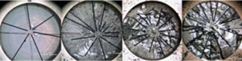
Project: Bistable links improve effectiveness of protective structures
Click on either of the following images to see an animation.

The first structure is a regular lattice of breakable links, while next one, which successfully repels the projectile, consists of the same mass of links that are “bistable” meaning that they have a first breaking point followed by a backup link recovery, which allows damage to be better spread through the structure rather than being focused at the impact point. By encouraging damage diffusion, the failure is no longer exclusively at the point of impact, as seen below by the red partially damaged bistable links. Continue reading
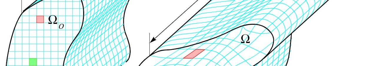
Streamline visualization of tensor fields in solid mechanics

Stress net view of maximum shear lines inferred from molecular dynamics simulation of crack growth. Image from http://doi.ieeecomputersociety.org/10.1109/VIS.2005.33

Brazilian stress net before and after material failure. Colors indicate maximum principal stress (showing tension in the center of this axially compressed disk). Lines show directions of max principal stress.
A stress net is simply a graphical depiction of principal stress directions (or other directions derived from them, such as rotating them by 45 degrees to get the maximum shear lines.) Continue reading
Annulus Twist as a verification test
Illustrated below is the solution to an idealized problem of a linear elastic annulus (blue) subjected to twisting motion caused by rotating the T-bar an angle 
This simple problem is taken to be governed by the equations of equilibrium 
Funding: CSM group receives $1.1M aimed at military vehicle safety

Stills from YouTube video of buried roadside explosive
As one of four institutions collaborating with the University of Colorado — Boulder, the CSM group in the Department of Mechanical Engineering at the University of Utah, will be developing constitutive models for soils, as well as full-scale simulation capabilities in Uintah to predict blast and ejecta from shallow buried explosives (such as roadside improvised explosive devices). The $1.1M slated for CSM work presumes the project will last 5 years. For more information, see the University of Colorado’s press release.
Exact solution for eigenvalues and eigenvectors/projectors of a real 3×3 symmetric matrix

The Pi (or Pie) Plane showing the region of the principal solution for the Lode angle and hence the region nearest the max eigenvalue.
It probably isn’t surprising that an exact solution can be found for eigenvalues of a real 3×3 symmetric matrix. This conclusion follows from noting that the characteristic equation is cubic, for which an exact solution procedure can be found in any good algebra reference. One thing that you won’t find in many such resources, however, is an algorithm for the solution that will avoid complex numbers in the intermediate steps of the calculation whenever the components of the source symmetric 3×3 matrix are all real.
